Study on Maximum Power Limitation of Gillnet Fishing Vessels Based on EEXI

Introduction

The horsepower of fishing vessel power units determines the vessel’s speed and fishing capacity, key factors affecting fishing vessels’ economic efficiency and energy consumption levels.^1,2 Excessive power configurations can lead to overfishing, exacerbating pressure on fishery resources and the marine ecological environment.^3–7 Therefore, scientifically and reasonably, determining the maximum power limitation of fishing vessels is of great significance for energy conservation, emission reduction, resource conservation, and sustainable fishery development. Properly setting the power systems of fishing vessels is crucial for optimizing their economic and environmental performance.

The International Maritime Organization (IMO) has focused on the energy efficiency of ships and has adopted mandatory energy efficiency standards such as the “2022 Guidelines on the Method of Calculation of the Attained Energy Efficiency Index (EEXI) for Existing Ships”,⁸ the “2022 Guidelines on the Method of Calculation of the Attained Energy Efficiency Design Index (EEDI) for New Ships”,⁹ and the revised “Annex VI of the MARPOL Convention” in 2021.¹⁰ However, these standards mainly target large commercial vessels, and there is a lack of systematic research on fishing vessels.^10–14 China has issued a “dual control” policy for fishing vessels, strictly controlling the total number and power of fishing vessels, gradually phasing out old and high-energy-consuming fishing vessels, and promoting the development of efficient and environmentally friendly fishing vessels.¹⁵ However, there is a lack of quantitative standards for the maximum power limitation of individual vessels. This reveals the urgent need to establish energy efficiency standards for fishing vessels.

Scholars at home and abroad have conducted fruitful research in ship energy efficiency optimization,^16–19 energy-saving technologies,^20–24 and operational management.^25–27 Han Xu(2021) et al.²⁸ used data visualization and machine learning methods to analyze and visualize the energy efficiency data of two 2,400 TEU container ships, identifying the main factors affecting speed and power. Zhou Kunxin et al. (2022)²⁹ proposed an optimization method based on an adaptive particle swarm algorithm, significantly improving the energy efficiency of the “Offshore Oil 301” vessel through power and speed optimization. Li Zongtao (2023) et al.³⁰ proposed a power decoupling-based energy efficiency maximization strategy (improved EEMS), significantly improving ship hybrid energy systems’ hydrogen fuel utilization rate. To address marine pollution and climate warming, China should enhance ship energy efficiency by optimizing main engine power, economic speed, and new propellers.³¹ Fishing vessels, in particular, significantly impact environmental pollution emissions, requiring attention and effective emission reduction measures.² This indicates that optimizing the energy efficiency of fishing vessels is an important way to achieve environmental protection.

China’s marine fisheries and total fishing vessel power have not been effectively controlled, and the phenomenon of “high horsepower” in small and medium-sized fishing vessels remains prevalent.^32,33 The issue of excess power in fishing vessels not only leads to overfishing but also affects the protection of fishery resources and the ecological environment,^1,7 necessitating research on the maximum power limitation of fishing vessels. This study aims to construct an EEXI reference line formula for fishing vessels, taking gillnet fishing vessels as an example, based on the energy efficiency standards of large commercial vessels. By combining the EEXI calculation formula, the reference line formula, and the power-speed relationship, the maximum power calculation formula for fishing vessels is derived. Addressing the issues of incomplete fishing vessel data records and the difficulty in applying the maximum power calculation formula, the study uses Decision Tree Regression, Random Forest Regression, and Gradient Boosting Regression methods to establish prediction models for the maximum power limitation of fishing vessels. Extensive analysis and research are conducted on the technical theory and practical applications of fishing vessel power limitation, constructing prediction models and calculation methods for the maximum power limitation of fishing vessels and providing recommendations for reducing fishing vessel power. This study offers new insights and decision-making references for enhancing fishing vessel power control and promoting green development in the industry. This emphasizes the importance of scientific research on power management of fishing vessels for the sustainable development of the industry.

Materials and Methods

Calculation of the EEXI Value for Gillnet Fishing Vessels

According to the “2022 Guidelines on the Method of Calculation of the Attained Energy Efficiency Index (EEXI) for Existing Ships” and the “2022 Guidelines on the Method of Calculation of the Attained Energy Efficiency Design Index (EEDI) for New Ships,” the EEXI and EEDI for different types of large commercial vessels have been specified, with the EEXI serving as a supplement and extension of the EEDI. The EEXI calculation formula is as follows, with units in (g/t•nm):

\[\small \begin{gathered} E E X I=\frac{A+B+E-D}{f_i \cdot f_c f_i \cdot \text { Capacity } \cdot V_{r e f} \cdot f_w \cdot f_m} \\ A=\left(\prod_{j=1}^n f_j\right)\left(\sum_{i=1}^{n M E} P_{M E(i)} C_{F M E(i)} S F C_{M E(i)}\right) \\ B=P_{A E} \cdot C_{F A E} \cdot S F C_{A E} \\ E=\left(\prod_{j=1}^n f_j \cdot \sum_{i=1}^{n P T I} P_{P T I(i)}+\sum_{i=1}^{n e f f} f_{\text {eff }(i)} \cdot P_{A E e f f(i)}\right) \cdot G \\ D=\sum_{i=1}^{n e f f} f_{\text {eff }(i)} \cdot P_{\text {eff }(i)} \cdot C_{F M E} \cdot S F C_{M E} \\ G=C_{F A E} \cdot S F C_{A E} \end{gathered}\tag{1} \]

In the formula, f_i，f_c，f_l，f_w，f_m，f_eff are coefficients used for correcting for technical/regulatory limitations on transport capacity, capacity correction coefficient, the coefficient for general cargo ships with cranes and other cargo-handling equipment, sea margin coefficient, IA Super and IA ice-class ship coefficient, and the coefficient for each innovative energy efficiency technology, respectively. Generally, f_i，f_c，f_l，f_w，f_m，f_eff are all set to 1. Capacity is the measure of the ship’s transport capacity, which is either deadweight tonnage (DWT) or gross tonnage (GT), depending on the ship type. For example, ro-ro ships and container ships use DWT as the measure of transport capacity, while cruise ships with non-conventional propulsion use GT.\(V_{ref}\) is the ship’s speed (in knots) in calm water conditions and at its corresponding carrying capacity in deep water.。\(C_{F}\) is the carbon conversion factor. SFC is the fuel consumption rate (in g/kWh), \(P_{ME}\) is the main engine power (in kW). If there are shaft motors, PPTI(i) represents 75% of each shaft motor’s rated power consumption divided by the generator’s weighted average efficiency, which is one of the innovative technologies. n is the number of main engines. The subscripts ME and AE represent the main and auxiliary engines, respectively. Together, these coefficients determine the total energy efficiency and carbon emissions of the vessel and are key factors in achieving environmental protection and energy efficiency management for ships.

Due to gillnet fishing vessels’ traditional and outdated equipment, innovative technology factors are not considered. Additionally, because their operational characteristics mainly involve accommodating large catches, using GT to measure carrying capacity aligns better with their actual operational needs.^8,9,34 This measurement method more accurately reflects the operational efficiency and capacity advantages of fishing vessels. Therefore, referring to the EEXI calculation formula for commercial ships, the EEXI calculation formula for gillnet fishing vessels is established as follows:

\[\small E E X I=\frac{P_{M E} \cdot C_{F M E} \cdot S F C_{M E}+P_{A E} \cdot C_{F A E} \cdot S F C_{A E}}{G T \cdot V_{r e f}} \tag{2}\]

Referencing the 2021 revised Annex VI of the MARPOL Convention,¹⁰\(C_{F}\)=3.114，SFC_ME=190(g/kWh)，SFC_AE=215(g/kWh).According to the “2022 Guidelines on the Method of Calculation of the Attained Energy Efficiency Index (EEXI) for Existing Ships” and the “2022 Guidelines on the Method of Calculation of the Attained Energy Efficiency Design Index (EEDI) for New Ships”,^8,9 \(P_{ME}\) is 75% of the total rated installed power (MCR_ME) of each main engine (i)^8,9，\(P_{AE}\)is 5% of the total rated installed power (MCR_ME) of each main engine (i)^8,9。These parameters and standards form the computational basis for ship energy efficiency assessment and management.

EEXI Reference Line Formula for Gillnet Fishing Vessels*

Due to the 2021 revisions of Annex VI of the MARPOL Convention, the EEXI reference line formula is specified in the following form:

The reference line formula is expressed as:

\[ R L V=a \cdot { Capacity }^{-b}\tag{3} \]

The expression for the required Energy Efficiency Existing Ship Index (EEXI) for existing ships is:

\[ Required\ EEXI\ =\left(1-\frac{Y}{100}\right) \cdot R L V\tag{4} \]

Formula 4 calculates the required EEXI value for existing ships as stipulated by the IMO, where Y is the reduction factor.

Data from over 5,000 gillnet fishing vessels from three coastal provinces were collected. Using Formula 2, their EEXI values were calculated, resulting in EEXI values corresponding to these vessels’ gross tonnage (GT). The dataset was then split into a training set and a test set in an 8:2 ratio [35] to fit the reference line formula. Subsequently, using the nonlinear least squares method, the gross tonnage (GT) and EEX values were fitted according to the reference line formula in the form of Formula 3, leading to the derivation of the EEXI reference line formula for gillnet fishing vessels.

Establishing the Calculation Formula for Maximum Power of Gillnet Fishing Vessels

The relationship between the total rated power of fishing vessels and their speed is evaluated as follows^35,36:

\[ V=1.84 *\left(\frac{P}{\Delta}\right)^{0.237} \sqrt{L}\tag{5} \]

Where V is the speed (in knots),P is the total rated power (in kW), \(\mathrm{\Delta}\) is the design displacement (in tons), and L is the length between perpendiculars of the fishing vessel (in meters).

The IMO stipulates that the EEXI of a vessel must be less than or equal to its reference line value. Therefore, by combining the EEXI calculation formula for gillnet fishing vessels (Formula 2), the reference line formula (Formula 3), and the power-speed relationship (Formula 5), it can be deduced that:

\[\frac{477.2205P}{GT \cdot 1.84*{(\frac{P}{\mathrm{\Delta}})}^{0.237}\sqrt{L}\ } \leq a{\cdot GT}^{- b}\tag{6}\]

When the EEXI reference formula for gillnet fishing vessels is fitted, thereby obtaining the values of parameters a and b, the relationship between the maximum power limit of the vessel and its gross tonnage, design displacement, and length between perpendiculars can be derived.

In this study, based on the standards of the International Maritime Organization (IMO), a set of Energy Efficiency Existing Ship Index (EEXI) calculation formulas suitable for gillnet fishing vessels was designed. By collecting the necessary data, the EEXI value of the gillnet fishing vessels was calculated, and using the reference line formula prescribed by the IMO, with gross tonnage as the independent variable and EEXI as the dependent variable, a reference line formula for gillnet fishing vessels was fitted. Further, the formulaic relationship between speed and power was incorporated into the EEXI calculations. According to IMO regulations, it is ensured that the EEXI calculation value derived from the speed-power relationship is less than or equal to the result calculated by the reference line formula, thereby deriving the maximum power calculation formula for gillnet fishing vessels, providing a scientific basis for the energy efficiency management of fishing vessels.

Regression Prediction of Maximum Power Limit for Gillnet Fishing Vessels

First, the maximum power values for over 5,000 gillnet fishing vessels are calculated using the relationship between the vessel’s gross tonnage (GT), design displacement, and length between perpendiculars (L). The dataset of over 5,000 vessels is then split into a training set and a test set in an 8:2 ratio. Regression prediction models are constructed with inputs consisting of GT and L, and outputs being the maximum power values.

During model training, Decision Tree Regression, Random Forest Regression, and Gradient Boosting Regression models are used, with initial model construction employing their main default parameters. The key default parameters for each model are as follows:

Decision Tree Regression:

criterion='squared_error' 
(Mean Squared Error as the criterion)

splitter='best' (Choose the best split)

max_depth=None (No maximum depth limit)

Random Forest Regression:

n_estimators=100 (100 trees)

criterion='squared_error' 
(Mean Squared Error as the criterion)

max_depth=None (No maximum depth limit)

bootstrap=True (Using bootstrap samples)

Gradient Boosting Regression:

loss='squared_error' 
(Mean Squared Error as the loss function)

learning_rate=0.1 (Learning rate of 0.1)

n_estimators=100 (100 boosting stages)

subsample=1.0 (Using the entire dataset)

max_depth=3 (Maximum tree depth of 3) 

Using these default parameters ensures the basic performance of the models and provides a benchmark for subsequent parameter optimization and tuning.By using three different regression models: decision trees, random forests, and gradient boosting, this study provides multiple methods for predicting the maximum power of fishing vessels.

Decision Tree Regression: Constructs the tree by recursively splitting the dataset into different subsets. Each node splits the dataset based on a threshold of a certain feature until stopping conditions are met. Advantages include:

Simple and intuitive structure, easy to interpret and visualize.

No need for data preprocessing.

Ability to handle both numerical and categorical data.

With its simple and intuitive structure, the decision tree model offers an easy-to-understand and implemented method for data partitioning.

Random Forest Regression: Improves accuracy and robustness by combining the predictions of multiple decision trees, each trained on random subsets and using random features for splitting. Advantages include:

High accuracy, reducing overfitting through ensemble learning.

Resistance to overfitting.

Ability to evaluate feature importance, aiding feature selection and data understanding.

With its advantages in ensemble learning, Random Forest regression excels in accuracy and robustness.

Gradient Boosting Regression: Incrementally builds tree models to optimize the objective function, with each tree trained on the residuals of the previous tree. Advantages include:

High performance, especially with complex datasets.

Flexibility in optimizing various loss functions.

Incremental improvement, enhancing prediction accuracy through iterative residual optimization.

Gradient boosting regression significantly improves prediction accuracy for complex datasets through iterative optimization.

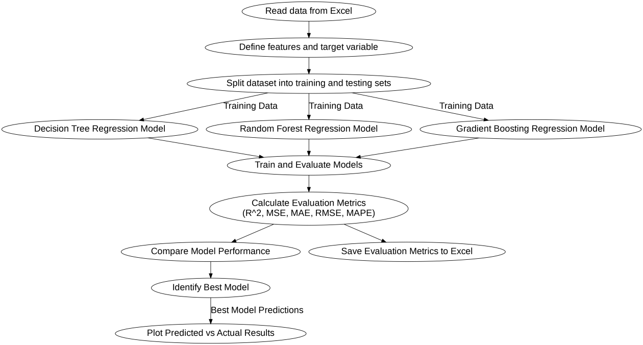
The models are trained and evaluated using metrics such as R², Mean Squared Error (MSE), Mean Absolute Error (MAE), Root Mean Squared Error (RMSE), and Mean Absolute Percentage Error (MAPE). The performance of the models on both the training set and the test set is assessed. Finally, by comparing the performance metrics of each model, the optimal model is determined. The process of establishing the regression prediction model for the maximum power limit of gillnet fishing vessels is outlined as follows.

Figure 1.Flowchart of the maximum power limit prediction model establishment

Results

Analysis of Baseline Formula Fitting Results

The EEXI values are calculated using the EEXI calculation formula. Some of the results are shown in Table 1.

The following reference line formula is obtained using the nonlinear least squares method to regress the gross tonnage and EEXI values according to the form of the reference line formula.

\[RLV = 1222.5311{\cdot Capacity}^{- 0.6075}\tag{7}\]

Its fitting degree is 0.6366. This indicates that the model can explain 63.66% of the variability in the data, thereby validating the significant correlation between the selected variables and the dependent variable. This high level of fit reflects the consistency between the model and the actual data and emphasizes its practicality in prediction and decision support, providing a solid foundation and direction for further research. The error evaluation metrics on the training set are as follows: MSE, MAE, RMSE, and MAPE are 87.2744, 6.1627, 9.3421, and 0.1279, respectively. On the test set, the error evaluation metrics are MSE, MAE, RMSE, and MAPE, which are 369.5200, 13.3518, 19.2229, and 0.1827, respectively. Notably, MAPE is below 20% on both the training and test sets, indicating that the model has good generalization and robustness without overfitting.

Specifically, the low MSE and RMSE on the training set indicate that the prediction error between the predicted and actual values is small, demonstrating good fitting performance on the training data. The low values of MAE and MAPE further confirm the high accuracy of the model. Although the error metrics on the test set are higher than those on the training set, they remain within a reasonable range, particularly with MAPE being below 20%, which shows that the model performs reliably on unseen data.

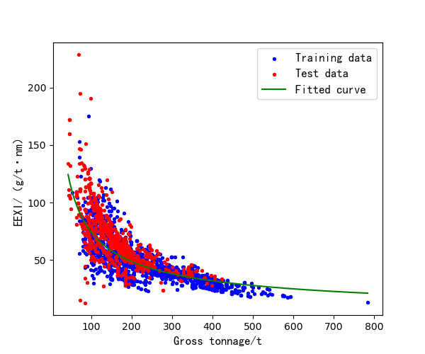
Combining the error evaluation results from both the training and test sets, it is evident that the model performs consistently across different datasets without significant performance fluctuations. This stability suggests that the model is adaptable in practical applications, effectively handling data prediction tasks in various scenarios. The fitting curve is shown in Figure 2, which illustrates the model’s fit to the data, further validating the analysis results of the error metrics. The diagram displays the relationship between two sets of data (labeled as ‘Training Data’ and ‘Test Data’) and a fitted curve (labeled as ‘Fitted Curve’). The diagram shows that as the variable on the horizontal axis increases, the variable on the vertical axis shows a clear downward trend. The training data (blue points) and the test data (red points) are distributed around the fitted curve, indicating that the model can accurately describe and predict this trend. The fitted curve smoothly approaches these two sets of data points, demonstrating the model’s good consistency and generalization ability across different datasets, which is crucial for verifying the model’s accuracy and practicality. The fitting curve indicates that the model can effectively capture data trends, demonstrating high predictive accuracy. The model demonstrates its effectiveness and robustness in practical applications through high fidelity and stable error performance across different datasets.

Figure 2.Fitting curve

Combining Equations 2, 5, and 7, the formula for calculating the maximum power of gillnet fishing vessels is derived as follows:

\[P_{MAX} = \ {(\frac{4.714 \cdot \sqrt{L} \cdot {GT}^{0.3925}}{\mathrm{\Delta}^{0.237}})}^{\frac{1}{0.763}}\tag{8}\]

Sensitivity Analysis of Various Factors on EEXI Values

A sensitivity analysis is performed on the EEXI values by varying the carrying capacity (GT), reference speed (Vref), and total rated power of the main engine (P) with change rates of -10%, -9%, -8%, -7%, -6%, -5%, -4%, -3%, -2%, -1%, 0, 1%, 2%, 3%, 4%, 5%, 6%, 7%, 8%, 9%, and 10%.Taking the vessel indexed as number 1 in Table 2 as an example, the sensitivity analysis results are shown in Table 2.

A lower EEXI value indicates better energy efficiency performance of the vessel. △EEXI represents the degree of change in the EEXI. Data from Table 2 shows that gross tonnage and speed have a comparable impact on EEXI, while power has a significantly larger effect. This implies that adjusting the power parameters is more effective in reducing the EEXI value than adjusting the gross tonnage and speed. Therefore, limiting the maximum power of gillnet fishing vessels is more advantageous for lowering their EEXI values, thereby significantly improving the energy efficiency of the vessels. By restricting the maximum power, fuel consumption and greenhouse gas emissions can be effectively reduced, and the lifespan of the engine and other equipment can also be extended, lowering maintenance costs. Power limitation policies can also encourage shipowners to adopt more efficient technologies and operational strategies, further enhancing overall energy efficiency. Therefore, by effectively managing and restricting ship power, the energy efficiency performance of ships can be directly and effectively improved, which has significant benefits for environmental protection and cost control.

Regression Prediction Model for Maximum Power of Gillnet Fishing Vessels

In the early stages, due to the imperfect data management in the fishing vessel domain, incomplete records of design parameters for fishing vessels were common. This made it difficult to apply the formula for calculating the maximum power of gillnet fishing vessels. Therefore, a regression prediction model was constructed using the gross tonnage and length between perpendiculars as input features, with the maximum power of gillnet fishing vessels as the output. First, the maximum power values for over 5,000 gillnet fishing vessels were calculated. The data was then split into training and test sets in an 8:2 ratio.³⁷ Decision tree regression, random forest regression, and gradient boosting regression models were used, with initial model construction employing their main default parameters. The performance evaluation metrics for the three models are shown in Table 3. Therefore, despite the challenges of incomplete data, by using advanced regression prediction models, researchers can still effectively estimate the maximum power of trawl fishing vessels, providing strong data support for ship design and energy efficiency improvements.

From the analysis of the data in Table 3, Table 4, and Table 5, it is evident that different regression models exhibit significant performance differences under various input variables. Although the Decision Tree model shows extremely high fitting accuracy on the training set, with an R² value close to 1, it exhibits clear overfitting on the test set, with large errors indicating insufficient generalization capabilities. In contrast, the Random Forest and Gradient Boosting models demonstrate more balanced performance on training and test sets, with smaller errors. The Random Forest model particularly shows stronger generalization ability and stability when handling nonlinear problems. Therefore, selecting the appropriate regression model requires careful consideration of the model’s fit and error on both the training and test sets, avoiding overfitting to ensure the model’s generalization ability.

The Random Forest model significantly reduces the risk of overfitting by integrating multiple decision trees and performs excellently under all input variable conditions, with the smallest errors on the test set, outperforming both the Decision Tree and Gradient Boosting models. Although the Gradient Boosting model also possesses strong generalization capabilities, its errors on the test set under different input variables are slightly higher than those of the Random Forest model. The random forest model effectively enhances the model’s generalization ability and prediction accuracy through ensemble learning, making it the best choice under various input variable conditions.

Considering the models’ fitting accuracy, generalization ability, and prediction accuracy, the Random Forest model outperforms the Decision Tree and Gradient Boosting models on both the training and test sets. Therefore, the Random Forest model is chosen as the final regression model.

Figure 3.Random Forest regression prediction effect of maximum power limit

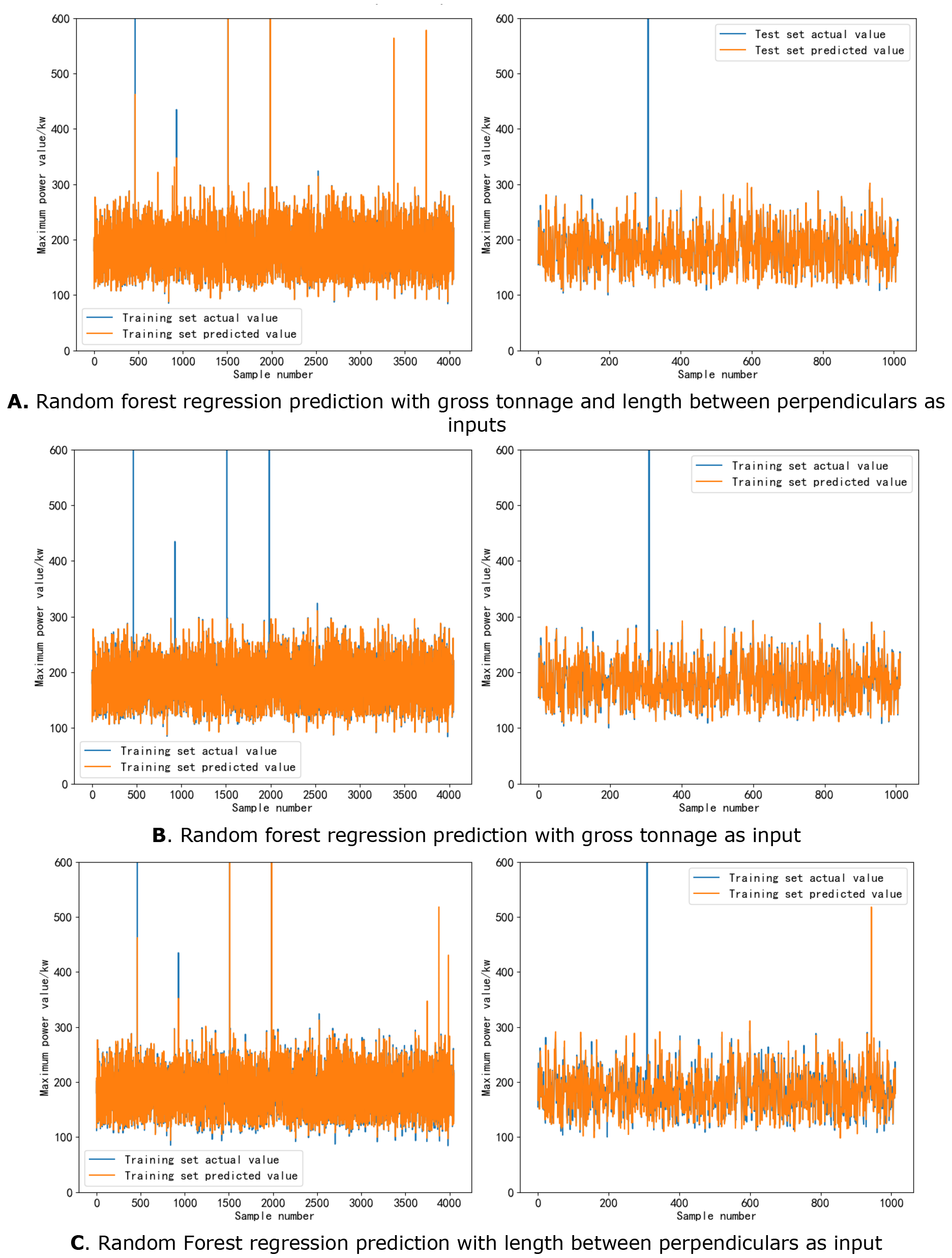
From the analysis of Figure 3 and the data in Table 3, Table 4, and Table 5, it can be seen that the performance of the Random Forest model varies significantly under different input variables. Specifically, the Random Forest model with gross tonnage and length between perpendiculars as input variables shows a large difference in MAPE (Mean Absolute Percentage Error) between the training and test sets, indicating overfitting. This suggests that while the model fits the training data well, it performs poorly on unseen data, showing insufficient generalization ability. Similarly, the Random Forest model with length between perpendiculars as a single input variable also exhibits similar issues, with significantly lower errors on the training set compared to the test set, further confirming the lack of robustness of the model. These results emphasize the importance of selecting appropriate input variables and avoiding overfitting using the random forest model.

In contrast, the Random Forest model with gross tonnage as the input variable shows a closer MAPE between the training and test sets, indicating better generalization ability and robustness. This model has more balanced errors on the training and test data, suggesting that it can predict accurately on known data and perform well on unknown data. Therefore, using gross tonnage as the input variable in the random forest model can effectively enhance the model’s generalization ability and prediction accuracy.

Considering the generalization ability, robustness, and prediction accuracy of the models, the Random Forest regression model with gross tonnage as the input variable is ultimately selected as the best model for predicting the maximum power limit of fishing vessels. By integrating multiple decision trees, the Random Forest model significantly reduces the risk of overfitting associated with a single decision tree model and performs excellently in handling nonlinear problems. In practical applications, its performance can be optimized by adjusting hyperparameters (such as the number and depth of trees), enhancing its predictive effect. In summary, the random forest model that uses gross tonnage as an input variable combines superior generalization ability and flexible adjustment mechanisms, making it an ideal choice for predicting the maximum power of fishing vessels.

Discussion

This paper thoroughly discusses the method for limiting the maximum power of fishing vessels and derives a predictive model for the maximum power of fishing vessels through theoretical analysis and empirical data calculation. The research results indicate that reasonable power limits are significant for improving the energy efficiency of fishing vessels and reducing emissions. The specific conclusions are as follows:

First, referring to the IMO energy efficiency standards, the EEXI formula for gillnet fishing vessels and the reference line formula were constructed. The sensitivity analysis indicated that power significantly impacts the energy efficiency of fishing vessels, providing a theoretical basis for subsequent power limit research. By developing the EEXI formula and conducting sensitivity analysis, this study provides a preliminary scientific basis for understanding and controlling the impact of fishing vessel power on energy efficiency.

Second, by combining the formula for the relationship between the total rated power and speed of fishing vessels with the EEXI reference line formula, the theoretical formula for the maximum power limit of fishing vessels was derived. It was confirmed that the maximum power value of fishing vessels can be effectively calculated based on parameters such as gross tonnage, design displacement, and length between perpendiculars, providing a quantitative standard for limiting the maximum power of gillnet fishing vessels. By deriving the formula and parameter analysis, this study has established a highly accurate method for calculating the maximum power of fishing vessels, laying a theoretical foundation for the practical application of power limitations.

Finally, decision trees, random forests, and gradient-boosting regression models were used to predict the maximum power of fishing vessels. The experimental results showed that the Random Forest regression model with gross tonnage as the input variable performed best in terms of robustness and generalization ability, providing a reliable prediction basis for the maximum power limit of fishing vessels. Considering the model’s fit, generalization ability, and prediction accuracy, the overall performance of the random forest model on both the training and testing sets is superior to that of the decision tree and gradient boosting models. The random forest model effectively addresses the issue of overfitting, primarily due to its method of constructing multiple decision trees and averaging their results, which enhances the model’s performance on unseen data. In contrast, although the decision tree model is easy to understand and implement, it is prone to overfitting due to slight changes in data; while the gradient boosting model can provide higher prediction accuracy in some cases, its training process is more complex and sensitive to parameter adjustments. Therefore, based on these considerations, the random forest model is selected as the final regression model because it provides stable generalization ability and maintains high prediction accuracy, making it suitable as a tool for predicting the maximum power of fishing vessels in this study. Ultimately, with its superior generalization ability and stable predictive performance, the random forest model becomes the most suitable regression model for this study.

In summary, this paper constructs a calculation method for the maximum power limit of fishing vessels through theoretical analysis and empirical research and verifies its effectiveness and application value. This research provides a systematic technical roadmap and decision reference for the sustainable development of the shipbuilding industry. The research findings on the maximum power limitation of trawl fishing vessels based on the Energy Efficiency Existing Ship Index (EEXI) can be applied to actual ship management and policy formulation through the development and implementation of relevant policies, ship design, and retrofitting, installation of monitoring systems, and ensuring compliance. This includes providing guidance for retrofitting existing vessels to meet energy efficiency and emission standards while improving operational efficiency and maintaining best practices through crew training and continuing education. Additionally, ship efficiency can be continuously optimized by regularly analyzing performance data and technological upgrades. These measures will help ship operators comply with new regulations while promoting sustainable development and environmental protection in the fishing industry.

In future studies, the selected random forest model can be further optimized, or other advanced models can be considered to enhance predictive performance in several ways. Firstly, for the random forest model, performance can be enhanced by adjusting the number of trees, depth, and other parameters, conducting more refined feature engineering, or employing advanced ensemble techniques. Simultaneously, exploring deep learning methods such as Multi-Layer Perceptrons (MLP) or Convolutional Neural Networks (CNN) and other models like Support Vector Regression (SVR) may exhibit better performance in handling complex relationships. Finally, enhancing the model’s interpretability and developing visualization tools can help researchers and users better understand and trust it, facilitating its effective deployment and use in practical settings. Through these comprehensive measures, future research will improve the model’s accuracy and applicability and enhance its acceptability and practical value.

Authors’ Contribution

Funding acquisition: Chao Lyu (Equal), Shanshan Zhu (Equal), Shuang Liu (Equal). Resources: Chao Lyu (Equal), Shanshan Zhu (Equal), Shuang Liu (Equal). Supervision: Chao Lyu (Equal), Shanshan Zhu (Equal), Shuang Liu (Equal). Conceptualization: Shanshan Zhu (Lead). Methodology: Shanshan Zhu (Lead). Formal Analysis: Shanshan Zhu (Lead). Investigation: Shanshan Zhu (Lead). Writing – original draft: Shanshan Zhu (Lead). Writing – review & editing: Shanshan Zhu (Lead).

Competing of Interest – COPE

No competing interests were disclosed

Informed Consent Statement

All authors and institutions have confirmed this manuscript for publication.

Data Availability Statement

All are available upon reasonable request.