Morphological variation of endemic Gymnocypris chilianensis (Cyprinidae) collected from three inland water systems in Qilian Mountains, China

Introduction

Gymnocypris chilianensis (Schizothoracinae, Cyprinidae) was first named by Li and Zhang (1974) during a fish survey in the Hexi Corridor area.¹ The distribution of G. chilianensis is narrow, distributed only in the three rivers in Qilian Mountains, China, including Shiyang River, Heihe River, and Shule River.¹ In recent years, due to changes in the ecological environment, construction of water conservancy projects, and overfishing, the habitat of G. chilianensis has been severely damaged, resulting in a sharp decrease in wild resources.² Therefore, the protection of its wild germplasm resources is particularly important. Based on this point, it is a key protected wild fish species in the Qilian Mountains, China. Meanwhile, it is also an important economic fish species in this era. At present, there is relatively little biological research on the G. chilianensis. Most research focuses on domestication, artificial breeding, and gender differences analysis; there have been no reports on the morphological differences between geographical populations of G. chilianensis. Some scholars believed that the G. chilianensis was a subspecies of the G. eckloni, and there was controversy over whether it was an independent species.³ Based on various molecular evidence, it is shown to be an independent species.⁴ For the convenience of description, this article expresses the G. chilianensis uniformly.

Many factors may influence the processes of species and phenotypic diversification. Morphologic differentiation expressed in phenotypic plasticity is an adaptation of the species in the environment.^5,6 Many fish adapt to their environment by reducing energy consumption during swimming. For example, the speed of water flow is an environmental factor affecting the shape changes of fish bodies and heads.⁷ In contrast, the shape can be changed to achieve unstable swimming efficiency in still water.⁸ In addition, survival pressure and selection pressure can also affect the morphological characteristics of fish.^9–11

Morphological research contributes to the identification and classification of germplasm resources.¹² The classification system, genus division, and geographic population definition of organisms rely on morphology as a basis.¹³ The methods adopted by the author of this article are divided into the truss network method and the landmark method.

Many studies on the differences between geographical groups use fish morphological characteristics. For example, researchers have found morphological differences in populations of Marbled Eel (Anguilla marmorata),¹⁴ Mediterranean horse mackerel (Trachurus mediterraneus),² Bloater (Coregonus hoyi),¹⁵ Terapon jarbua,¹¹ Nile perch (Lates niloticus),¹⁶ Coilia nasus,¹⁷ Clupisoma garua.¹⁸ In summary, traditional morphology and framework methods have become commonly used in taxonomic research and are important for studying fish morphology. Therefore, this study uses the framework model method combined with the traditional morphological characteristics, focusing on the Shiyang River, Heihe River, and Shule River, where G. chilianensis is mainly distributed in the Qilian mountains.

The morphological variation of G. chilianensis reflects their adaptability under different environmental conditions and ecological strategies during evolution, which helps us better understand the diversity of different populations of G. chilianensis and their importance in the ecosystem. Selecting three sampling sites in the Shiyang River basin and the Shule River basin and four sampling sites in the Heihe River basin to determine the morphological differences between populations and divide different groups reveals the population composition characteristics and benefits for fine management, thus providing accurate support for the resource dynamic changes of G. chilianensis and resource conservation.

Materials and Methods

Sample Collection and Preparation

All morphological indexes were observed and measured on 191 individuals of G. chilianensis. Collected from water bodies in ten sampling sites of three river basins (Shiyang River Basin, Heihe River Basin, and Shule River Basin) in Qilian Mountains, China (Figure 1 and Table 1) from July to August 2023. Given that the G. chilianensis is only narrowly distributed in these three river systems—the Shiyang, Heihe, and Shule River Basins¹⁹—We sampled from these three rivers and chose sites from the upper, middle, and lower regions of each to collect samples (three to four points for each river), thereby ensuring comprehensive coverage of the species’ distribution range.

Figure 1.The geographic coordinates of the sample location.

At the same time, record the sampling latitude and longitude of each geographical group and ensure that individuals are undamaged during sampling.

Sample processing and measurement

After sampling, the samples were placed on the experiment table in the field, the digital camera (model: SM-S9180) was fixed at 50 cm away from the experiment table, the focal length was fixed in the appropriate light environment for shooting, and two side photos of each sample fish were taken at the same angle for geometric analysis.²⁰The same experimenter completed all the above operations, thereby minimizing the errors caused by human operation.²¹

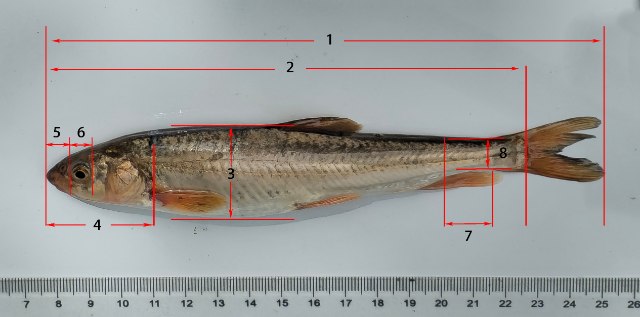
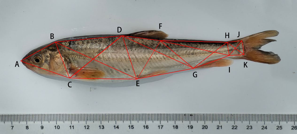
The traditional morphology and geometric morphology data of G. chilianensis were measured by using a ruler (± 0.01mm) and Digimizer application (version 5.4.4), and the body mass (± 0.01g) was measured by electronic balance. Using traditional morphological measurement methods (Figure 2),^22,23 8 measurable traits, including total length (TL), body length (BL), body height (BH), head length (HL), snout length (SL), eye diameter (ED), caudal peduncle length (CPL), and caudal peduncle height (CPH) were measured using a vernier caliper (± 0.01mm). A total of 11 coordinate points from A to K are selected on the side of the sample, and 23 frame parameters are measured (Figure 3),²² including AB,AC,BC,BD,CE,DE,CD,DE DF,EG,DG,EF,FG,FH,GI,FI,GH,HI,HJ,IK,HK,IJ,JK were measured with Digimizer program.

Figure 2.Traditional morphological measurement of G. chilianensis

(1. Total Length-TL; 2. Body Length (BL); 3. Body Height (BH); 4. head length (HL); 5. snout length (SL); 6. eye diameter (ED); 7. caudal peduncle length (CPL); 8. caudal peduncle height (CPH)).

Figure 3.Geometric morphological measurement of G. chilianensis

(A. snout; B. the upper-end point of gill cover; C. the starting point of pectoral fin; D. the starting point of the dorsal fin; E. the starting point of ventral fin; F. the end of dorsal fin; G. the starting point of anal fin; H. the starting point of the upper lobe of caudal fin; I. the starting point of the lower lobe of caudal fin; J. the point of upper caudal fin base; K. the point of lower caudal fin base;).

Data Processing Analysis

To eliminate the influence of fish size difference and improve the data accuracy, the formula M_s=M₀(L_s/L₀) ^b was used for correction. Where MS=standardized measurement value, M₀=unit length of measurement, Ls=overall (arithmetic) average length of all fish in all samples, L₀=standard length of the sample, and b is each character estimated according to the allometric growth equation M=_aL^b based on the observed data.²⁴ Through the analysis of standardized multivariate data, statistical methods such as Principal Component Analysis (PCA) are employed to compare morphological patterns and discern the primary sources of variation in morphology.

After standardization, the variables of full length and body length are removed. 29 measurable traits were obtained after formula correction (Table 2). SPSS software was used to perform one-way ANOVA on the eigenvalues of the 29 measurable traits, and LSD and Tamhane′s T multiple comparisons were used to analyze the morphological differences among different populations.²⁵ Principal component analysis was performed on all morphological characteristics data of all populations to obtain the load value and contribution rate of each principal component, and the principal component dispersion map was drawn according to the score of the principal component with greater contribution. Cluster analysis was performed on 29 measurable traits corrected by 10 populations using the cosine distance coefficient because cosine distance has high efficiency in analyzing large datasets.²⁶ The clustering relationship diagram of 10 geographical populations was drawn.

Landmark data processing

Landmark points are selected within the morphological body structure of fish. Variations in body structure among different individuals can be discerned through these points. However, variations in the placement, orientation, and scale of punctuation on specimens can alter the relevance of direct analysis. Therefore, it is essential to eliminate the interference of non-morphological variation in the analysis. While several methods have been applied, they employ slightly differing theories and optimization principles. Currently, the overlay method remains the most widely used.²⁷ This experiment also uses the tps series program to establish landmark.²⁰ Use the tpsSmall program to measure the regression coefficient to verify the validity of landmarks and the tpsRelw program to calculate the mean morphology of landmarks in different sample groups. The tpsRegr program is used to analyze the landmarks that draw the grid diagram of the G. chilianensis in different sample groups and visualize the morphology difference.

Results

Analysis of Variance

One-way analysis of variance (ANOVA) was used to analyze the eigenvalues of 29 measurable traits of G. chilianensis from 10 populations (Table 3). The results showed that the differences in measurable traits among 10 populations were significant or extremely significant.

Principal Component Analysis

After standardization in different point populations, principal component analysis (PCA) was performed on the ratios of 29 measurable traits of all G. chilianensis. KMO and Bartlett test showed that KMO was 0.652>0.6, indicating that the data were suitable for factor analysis; Bartlett’s spherical significance P=0.00, indicating that this case variable can provide a reasonable basis for factor analysis. Results of eight principal components were extracted (Table 4), and the cumulative contribution rate of the eight principal components was 79.679%. The variance contribution rates of the first three principal components were 24.809%, 13.355%, and 10.061%, respectively, and the cumulative contribution rate was 48.225%.

The principal component analysis showed that (Table 5) the factor load value of principal component 1 ranged from -0.443 to 0.771, and the ratios of measurable traits greater than 0.7 were M14, M24, M27, M28, which were mainly concentrated in the morphological differences of the trunk and tail of the fish. The factor load value of principal component 2 ranged from -0.525 to 0.706, and the ratios of measurable traits greater than 0.6 were M7 and M8, mainly concentrated in the morphological differences of the head and caudal fin. The load values of the principal component 3 factors ranged from -0.240 to 0.760, and the ratios of measurable traits greater than 0.6 were M10, M12, and M13, which were mainly related to the morphological differences of the trunk parts of fish. The head and tail exhibit significant load on the first three principal components, suggesting that evolutionary forces may primarily act on these regions.

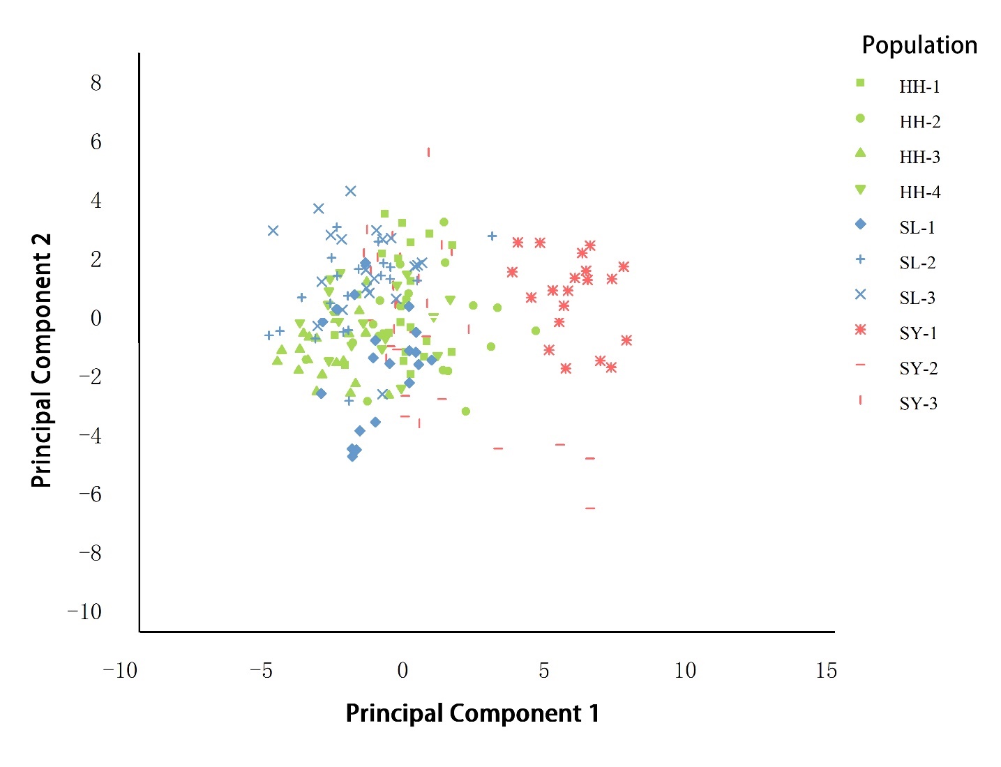
A scatter plot is constructed using the first and second principal components (Figure 4). To facilitate distinction, points within the same watershed are represented by the same color in Figure 4. The scatter plot reveals that the Heihe River basin, situated in the central region, and the Shule River basin, located in the western part, are densely distributed and overlap in their distribution patterns. The boundaries between these groups are not distinct, suggesting that the individual features of the Heihe River and Shule River basins are relatively similar. The distribution of the Shiyang River basin located in the east is relatively independent, and the individuals in the Shiyang River basin are different from the other two basins.

Figure 4.Scatter plot of the first and second principal components of ten different G. chilianensis populations.

Cluster Analysis

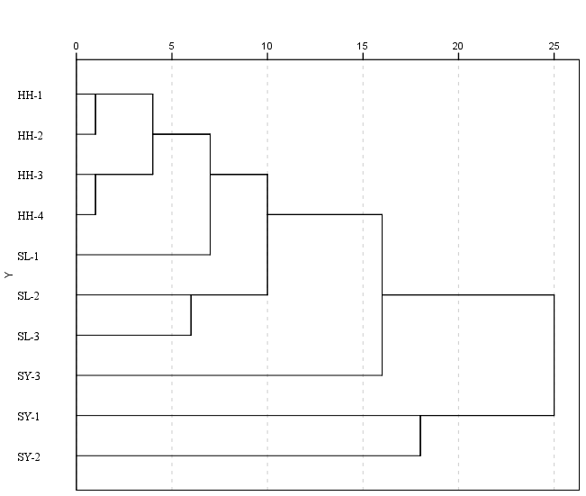
The clustering analysis results are shown in Figure 5. Determine the clustering threshold based on the elbow rule; thresholds can effectively categorize individuals, which greatly aids in the clustering of groups at the distance of 5; the four groups of the Heihe River basin gathered into one branch. At a distance of 15, 10 different geographical groups are divided into three clusters: HH-1, HH-2, HH-3, HH-4, SL-1, SL-2, and SL-3, and grouped together. SY-3 is an independent group, while SY-1 and SY-2 are combined together. The results showed that the populations in the Heihe River and Shule River were significantly clustered, while the population in the Shiyang River was distributed in another group. This indicates that the populations in the Heihe River and Shule River are relatively similar, while there are significant differences between the Shiyang River and the other two basins. In addition, the populations of SY-3 and the other two points in the Shiyang River did not cluster together, indicating significant genetic differences and distant genetic relationships between populations in the same basin of the Shiyang River, which is consistent with the results of the principal component analysis.

Figure 5.The pedigree chart among the populations of G. chilianensis

Discriminant Analysis

Stepwise discriminant analysis was conducted on 29 morphological proportional traits in 10 populations, and 12 feature values with high contribution rates were selected: M3, M4, M8, M9, M10, M12, M13, M16, M19, M21, M28, M29. These were used for stepwise discriminant analysis of morphological variables in different populations of G. chilianensis and to construct discriminant equations for each population. The main results are shown in Table 6.

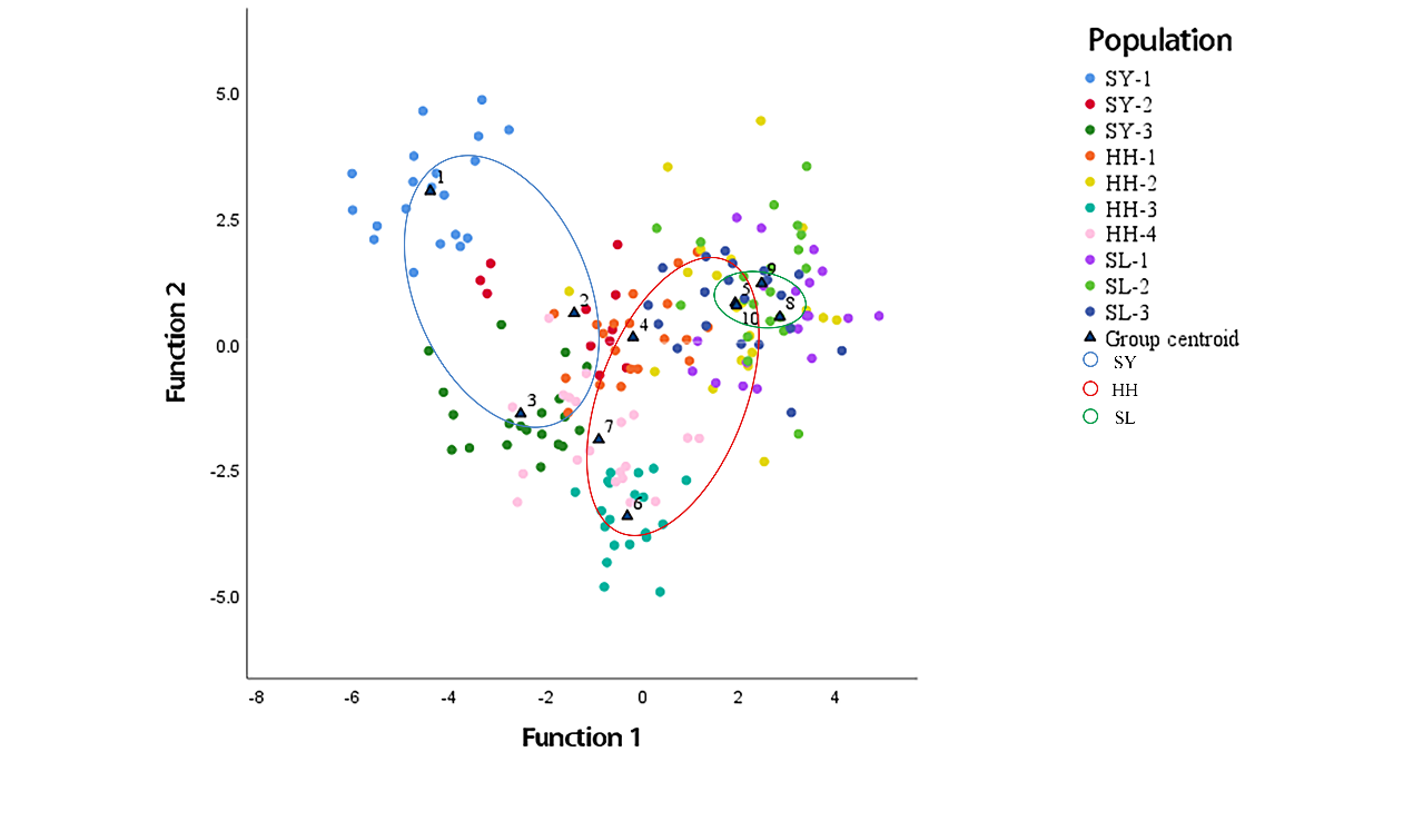
The discriminant analysis results (Table 7) indicated that the stepwise discrimination achieved a comprehensive discriminant rate of 95.30%, while the cross-validation produced a rate of 84.30%. SY-1 demonstrated the highest accuracy of 100% in both stepwise discrimination and cross-validation. The accuracy of discrimination for SL-1 is low. The scatter plot of discriminant analysis showed that the Shiyang River populations were largely separated from the other two populations, consistent with the cluster analysis results. The overlap between Heihe River and Shule River points is large, indicating similar morphology.

Landmark Difference Visual Analysis

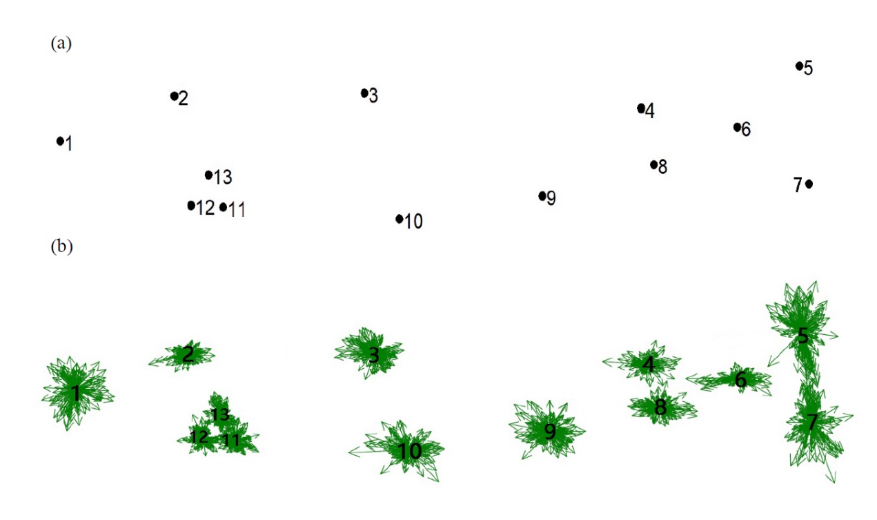
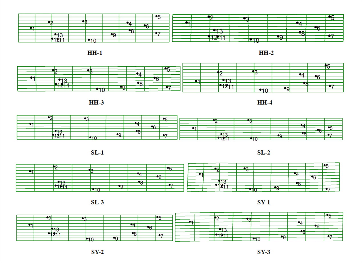
Using the tps series program, the tpsDig2, to choose 13 landmarks and verify the regression coefficient by the tpsSmall to get the regression coefficient greater than 0.99, it’s proved that the selected landmarks are valid. Overlap effect of vectorization of mean shape and all landmarks of different G. chilianensis populations in Figure 6, most differences are embodiment in 1, 5, 7, 10 points, mouth, pelvic fin, and caudal fin. By vectorization and meshing mean shape in Figure 7, most differences are embodiment in 3, 5, 6, and 7, where there are the trunk and caudal fin.

Figure 6.Discriminant function analysis for morphological traits in ten populations of G. chilianensis.

Figure 7.Overlap effect of vectorization of mean shape and all landmarks of different G. chilianensis populations. (a. average shape of G. chilianensis; b. overlapping effect of vectorization of all landmarks and 1-19 landmarks. ）

Figure 8.Mesh deformation maps of 10 populations of G. chilianensis (variation enlargement by 10 times).

Discussion

Based on the truss network method and landmark method, 29 measurable traits were compared and analyzed among 10 geographic populations, effectively contrasting the trait differences between individuals. This method has the advantages of simple operation, high efficiency, minimal damage to fish bodies, and significant comprehensive effects.²⁸

Cluster analysis classifies different groups, directly reflecting the size of differences between groups.¹³ The results show significant differences among the three river basin groups, and Shiyang River basin groups are the most different from other groups.

In this study, 29 morphological proportional traits were analyzed by cluster analysis, which reflected the similarity of morphological characteristics of the G. chilianensis populations at the overall level. According to the clustering results, the morphological differences in distance among populations in the Heihe River basin were the smallest, and then clustered into a large group with the Shule basin three populations at the distance of 10; SY-3 as a separate group SY-1 and SY-2 populations were clustered into one group respectively, and there were significant differences among the three groups, with large morphological differences and distant genetic relationships, which conformed the research laws that the same species with long geographical distances and geographical barriers may have large morphological differences.^28,29 In cluster analysis, in addition to slope, the Pearson correlation coefficient, Euclidean distance, and Chebyshev distance were also chosen for analysis. However, the results showed that cosine distance was more explanatory, and the Pearson correlation coefficient also yielded similar results. If you have any questions about the selection method, you can discuss it with the author later.

Landmark results show that the trunk and caudal fin had the most obvious characteristics. A similar finding is presented in some species, such as Coilia nasus.¹⁷ Principal component analysis can reflect the degree of morphological differences among different populations. In this study, 7 principal components were extracted, and the cumulative contribution rate was 80.752%. Generally, it is necessary to extract 85% of the common factor cumulative contribution to make sense, but the sample size of this study is large, and the common factor is extracted according to the cumulative contribution rate of more than 70%.³⁰ Principal component 1 mainly reflects the difference in caudal fin. The mean height of the caudal fin of the ten populations in descending order was: SY-1, SY-2, SY-3, HH-1, HH-2, HH-3, HH-4, SL-1, SL-3, SL-2, the population of Shiyang River is generally larger than that of the other two Rivers. This result once again proves that the population of Shiyang River differs significantly from the populations of the other two watersheds, while the other two populations are more similar.

Different populations grew and developed in different environments and were easily affected by the environment and selection pressure, resulting in environment-induced morphological variation.^31,32 On the contrary, morphological features can also be reversed to reflect the adaptation of fish to the environment^30.31.32. On the other hand, it may be related to the swimming ability of G. chilianensis; the swimming ability of fish can be described by durable swimming speed, sustained swimming speed, and explosive swimming speed.¹⁷ Explosive swimming is a short-term anaerobic exercise carried out by fish, mainly through their trunk and caudal fins, to engage in life activities such as foraging and avoiding enemies. It is an important swimming method for fish and occurs at every stage of life.³³ One of the most important morphological features of explosive swimming is its wide trunk and caudal fins.³²

The Shiyang River Basin has yielded a smaller number of individuals than other basins, with analyses revealing significant differences. It is hypothesized that the basin may have encountered bottleneck effects (such as droughts, floods, or human fishing), leading to a drastic reduction in the number of individuals. The genes of the surviving individuals differ markedly from the original population, leading to genetic drift in subsequent generations.³⁴ Additionally, the varied environmental conditions within rivers may have enhanced the adaptability of fish within their distinct environments, thereby increasing the likelihood of genetic drift.³⁵ Given that the strength of genetic drift increases as population size decreases, management activities have focused on increasing population size through preserving habitats to preserve genetic diversity.³⁶

The difference in tail reflects the adaptation of G. chilianensis to motion and maneuverability. The strong tail is a very important condition for the long-distance reproductive migration of G. chilianensis.³⁷ For the morphological differences of the G. chilianensis in different water systems (Shiyang River system, Shule River system, Heihe River System), the morphological variables related to tail differences were screened out in the first component of principal component analysis, showing significant tail differences. Based on this, the author believes that the differentiation may occur due to the different geographical locations of the three rivers and the great differences in the hydrological environment and natural environment.³⁸

The truss network can better compare the characteristics between ten different populations. The discriminant analysis and cluster analysis results are homogeneous, and a stable discriminant function is established by combining the best factor of stepwise discriminant analysis with the ability to screen variables.³⁹ The discrimination accuracy of the three populations in Shiyang River is the highest, with 100.00%, 90.00%, and 72.70%, respectively, proving that the degree of mixing is the lowest, significantly different from the other two populations. The discrimination accuracy of the three populations in the Shule River is lower, with 65.00%, 80.00%, and 75.00%, respectively, and the individuals who made discrimination errors in the Shule River basin are all considered to be from the Heihe River basin (Table 7.), which the unique geographical factors of Heihe River may cause. The upper reaches of the Heihe River are located in Qinghai Province on the other side of the Qilian Mountains, with high altitudes, and the vegetation in the basin is mainly grassland and river valley; numerous tributaries and rich water sources promote gene exchange among populations.³ The comprehensive discrimination rate of the discriminant function based on 29 main eigenvalues is 95.30%, which shows that the formula is reliable in distinguishing the differences in population characteristics. and the truss network can better compare the differences between different populations.

Based on these results, the differences between populations of the G. chilianensis in this study are mainly reflected in the differences in tail stalk and trunk. Among them, the caudal fin is the main variation direction in different populations of G. chilianensis, and the trunk is the secondary variation direction, mainly related to ecological habits such as habitat utilization and feeding. Among the three river basins, the differences between the populations in the Heihe River basin and the Shule River basin are relatively small, while the differences between the populations in the Shiyang River basin are the largest. It means that the population structure of the Heihe River and the Shule River basin are similar. Due to the differences between groups in the Shule River basin and the Heihe River basin are small, based on this, the Heihe River basin and Shule River basin can be managed as a unified group, while the Shiyang River basin can be managed as a separate group for more detailed management. Meanwhile, the more independent Shiyang River basin groups should be further analyzed in the next step to reveal the specificity of the three populations in this watershed.

This study provides an effective theoretical basis for the division and fine management of the protection of G. chilianensis germplasm resources, but there are still some limitations. Specifically, the morphological characteristics of fish are highly variable, and sometimes, these variations may be due to environmental changes rather than genetic relationships. Morphological changes are generally a slow process, and some features may respond to environmental changes but may not conform with the genetic outcomes. Additionally, there are other limitations as well. Consequently, it is necessary to combine these methods with molecular biology to distinguish more accurately between different populations to achieve this objective.

In the future, it is necessary to comprehensively explore the population composition and life history differences of the G. chilianensis population from multiple perspectives (such as otolith microchemistry, molecular biology, etc.). This can provide a theoretical basis for the function of the main river basins and the protection of the G. chilianensis germplasm resources.

Acknowledgments

We would like to thank Mr. Yong Qin for his assistance in collecting samples. This research is financially supported by the National Natural Science Foundation of China (32273140).

Authors’ Contribution

Data curation: Biyuan Liu (Equal), Qiqun Cheng (Equal). Formal Analysis: Biyuan Liu (Equal), Qiqun Cheng (Equal). Investigation: Biyuan Liu (Lead), Qiqun Cheng (Lead), Tai Wang (Lead), Zhongyu Lou, Di Peng, Dan Song. Resources: Biyuan Liu (Lead) , Qiqun Cheng (Lead), Zhongyu Lou, Tai Wang. Software: Biyuan Liu (Equal), Qiqun Cheng (Equal). Validation: Biyuan Liu (Lead), Qiqun Cheng (Lead), Zhongyu Lou, Di Peng, Tai Wang, Dan Song. Visualization: Biyuan Liu (Equal), Qiqun Cheng (Equal). Writing – original draft: Biyuan Liu (Lead). Writing – review & editing: Biyuan Liu (Lead), Qiqun Cheng (Lead), Zhongyu Lou, Di Peng. Methodology: Biyuan Liu (Lead), Qiqun Cheng (Lead), Zhongyu Lou, Di Peng, Tai Wang, Dan Song. Conceptualization: Qiqun Cheng (Lead). Funding acquisition: Qiqun Cheng (Lead). Project administration: Qiqun Cheng (Lead). Supervision: Qiqun Cheng (Lead)

Competing of Interest – COPE

No competing interests were disclosed.

Ethical Conduct Approval – IACUC

All animal experiments in this study followed the relevant national and international guidelines. The East China Sea Fisheries Research Institute’s Institutional Animal Care & Use Committee (IACUC) approved our project.

Informed Consent Statement

All authors and institutions have confirmed this manuscript for publication.

Data Availability Statement

All are available upon reasonable request.