Prediction of Shrimp Price Based on WOA-VMD-XGBoost Algorithm and SHAP Model

1. Introduction

In recent years, China’s aquatic products market has been developing rapidly, and the total and per capita consumption of aquatic products has been increasing yearly. Residents’ demand for and consumption of aquatic products is expected to increase further. Therefore, building a set of aquatic products price prediction systems adapted to the market environment and changing trends can not only provide aquaculture enterprises with rational planning of aquaculture structure, maximize aquaculture income, and effectively promote the sustainable development of aquaculture, but also provide a scientific basis for the government to formulate corresponding industrial policies and safeguard national food security.

Currently, research on fish price forecasting has made a big breakthrough. Statistical model-based forecasting methods, such as Peng D et al.¹ applied simple exponential smoothing (SES), Holt linear trend method, and Holt-Winters addition method to simulate and forecast scallop prices, and the results showed that the SES model had the highest forecasting accuracy. Nam and Sim² used ARMA model to forecast abalone prices, and the experiments showed high model accuracy. Junqi W and Xuecheng W³ used the model SARIMA model to predict the monthly price of shrimp in Lingjiatang area of Jiangsu Province for the next two years. Hasan et al⁴used the ARIMAX model to predict the price of catfish, and the results showed that the model had a high predictive performance.

The exponential smoothing method and ARIMA time series prediction model used in the above studies have low error tolerance and relatively poor prediction accuracy, and more scholars choose to use machine learning methods to construct price index prediction models. For example, Jin B, and Xu X⁵ constructed a non-linear autoregressive neural network to forecast the wholesale price index of agricultural products, and the research results show that the neural network model is better than the AR and GARCH (1,1) model. Singh N D et al.⁶ applied ANN model to predict the weekly price of shrimp export in India, and the predicted value was accurate and synchronized with the real data. Qingling D et al⁷ used a genetic algorithm to optimize the SVR model and predicted the price of Siniperca chuatsi fish and other aquatic products. The results show that the GA-SVR model is better than BP neural network, and the prediction accuracy is significantly improved. Nguyen et al⁸ applied random forest and gradient boosting tree algorithms to predict the price of exported aquatic products, and found that the gradient boosting tree algorithm is optimal for short-term prediction.Junhao W et al⁹ proposed a model that applies variational modal decomposition and deep learning to the prediction of aquatic product price, and the prediction accuracy is high. model with high prediction accuracy. Although the deep neural network has high prediction accuracy, it lacks the interpretation of the prediction results.¹⁰With the increasing popularity of interpretable machine learning, machine learning methods can extract unique insights from datasets with characteristic variables.¹¹Deng S et al¹² proposed a predictive model based on interpretable machine learning to predict the carbon price in the Hubei carbon trading market using the complete ensemble empirical mode decomposition with adaptive noise (CEEMDAN) and LightGBM-SHAP models. The results show that the high-frequency intrinsic mode function (IMF) component of the historical carbon price is the most important feature for predicting the carbon price trend.Khiem, N.M et al.¹³ used a super learner to predict the export price of shrimp from Vietnam and applied the SHAP model to analyze the key factors affecting the shrimp exported under Vietnam.

Compared with traditional machine learning models, Extreme Gradient Boosting (XGBoost) is an integrated learning algorithm and is widely used in the fields of finance, medicine, and engineering,¹⁴ which depicts the underlying mechanism between the input features and the target outcome and has the advantages of high prediction accuracy and less overfitting.¹⁵ However, there is less literature on applying variational modal decomposition (VMD), XGBoost algorithm and SHAP model to fish price prediction. Therefore, this study attempts to introduce the XGBoost machine learning algorithm into shrimp price prediction and integrate it with the Bayesian optimization (BO) algorithm to optimize the hyperparameters. The WOA-VMD model adaptively decomposes the price series to reduce the data noise. The decomposed trend term, period term, high-frequency term, low-frequency term, and residual term are used as inputs to the XGBoost regression algorithm for training and testing and combined with the SHAP model to analyze the nonlinear effects of key factors to provide scientific and effective methods and technical support for the relevant management departments and units to predict the consumer prices of aquatic products.

2. Materials and Methods

2.1. Principle of WOA algorithm

The Whale algorithm is a new population intelligence optimization algorithm created to find the optimal solution to the search problem. It was created by Mirjalili et al.¹⁶ in 2016 based on the hunting behavior of humpback whales. In the whale algorithm, the position of each whale represents a feasible solution. There are three types of position updates during whale group hunting: siege, attack, and search.

2.1.1. Siege

Individual whales will share information about their position where they have searched for the most prey, and then the whales will swim towards the one closest to the prey, causing the group to gradually complete the encirclement of the smaller group and narrow the encirclement circle, and the updating formula for the position of the whales during this hunting process is:

$$\overrightarrow{D_{1}} = \left| \overrightarrow{C} \cdot \overrightarrow{X^{*}}(t) - \overrightarrow{X}(t) \right|\tag{1}$$

$$\overrightarrow{X}(t + 1) = \overrightarrow{X^{*}}(t) - \overrightarrow{A} \cdot \overrightarrow{D_{1}}\tag{2}$$

Where $\overrightarrow{X^{*}}$represents the vector of prey positions, $\overrightarrow{X}$represents the vector of whale positions, t is the number of iterations.

2.1.2. Bubble Attack

Humpback whales, looking for prey as a spiral, will slowly approach the target and use a spiral bubble sent to capture prey, first calculate the distance between the whale and prey. The distance is used to generate the spiral equation, which is as follows:

$$\left\{ \begin{aligned} & X(t + 1) = X^{*}(t) + D \cdot e^{bl}cos(2\pi l) \\ & D = \left| C \cdot X^{*}(t) - X(t) \right| \end{aligned} \right.\ \tag{3}$$

where b is a constant and l is a random number between [-1, 1]. As humpback whales move around in the ocean looking for prey, the whales’ choice of seining and spiral bubbling to catch prey has a random nature, so to simulate this behavior, it is necessary to encircle the prey and spiral searching in tandem.

2.1.3. Search

To improve the overall search function of the whales, the stochastic nature of the whales in searching for food, and to improve the range of their search, a spiral search method was adopted. The updating formula for the random search position is

$$\begin{align} X(t + 1) &= X_{\text{rand }}(t) \\ &\quad - A \cdot \left| C \cdot X_{\text{rand }}(t) - X(t) \right| \end{align}\tag{4}$$

Where $X_{\text{rand }}$is a random position vector in a whale population. These three methods form a method based on optimal individual search (seining, bubble net) and arbitrary single (seining), which has better convergence and overall optimization performance.

2.2. Principle of VMD

Variational Modal Decomposition VMD is used to obtain modal functions with a certain wide frequency range by continuously updating each modal function and center frequency.¹⁷ The basic idea of VMD is to obtain the analytic signal by Hilbert transforming the mode components through the filtering model, shifting the spectrum of the mode components to the fundamental frequency by exponential mixing, and finally estimating the bandwidths of the mode components by H1 Gaussian smoothing.¹⁸ The corresponding constrained variational expression is.¹⁹

$$\small{\min_{\left\{ u_{k} \right\},\left\{ \omega_{k} \right\}}\mspace{2mu}\left\{ \sum_{k = 1}^{K}\mspace{2mu}\left. \parallel\partial_{t}\left\lbrack \left( \delta(t) + \frac{j}{\pi t} \right)*u_{k}(t) \right\rbrack e^{- j\omega_{k}t} \right.\parallel_{2}^{2} \right\}\tag{5}}$$

$$\text{subject to: }\sum_{k = 1}^{K}\mspace{2mu} u_{k}(t) = x(t)$$

where:$\delta(t)$is the Dirac distribution with respect to time t;$*$is the convolution operator; and $\omega_{k}$ is the center frequency of $u_{k}(t)$.

2.3. Principle of XGBoost Algorithm

The Extreme Gradient Boosting (XGBoost) algorithm is a comprehensive learning algorithm developed by Tianqi Chen et al. in recent years. It is an efficient implementation of Gradient Boosted Decision Tree (GBDT). Strong classifiers are constructed by integrating multiple weak classifiers, second-order Taylor expansion of the loss function,²⁰ along with the use of a regular term to prevent overfitting of the model,²¹ and training with an objective function. The algorithm’s math is as follows.²²

XGBoost uses the CART tree model, which can be viewed as predicting the structure of yi based on the input xi, with the formula:

$${\widehat{y}}_{i} = \sum_{k = 1}^{K}f_{k}\left( x_{i} \right),f_{k} \in F\tag{6}$$

where K is the number of trees, f_k is a function in the function space F, and F is the set of all possible CARTs. For the regression problem, the task of training the model lies in finding the best parameter θ that best fits the training data x_i and the outcome y_i. The objective function to be optimized is to measure the model’s fit to the data.

$$\ obj(\theta) = L(\theta) + \Omega(\theta)\tag{7}$$

Where Ω is the regularization term, which is related to the complexity of the tree;L is the training loss function, which is used to measure the model’s predictive ability, and the higher the prediction accuracy, the smaller L will be. A common choice is the mean squared error, given by the following equation.

$$\ L(\theta) = \sum_{i}^{}\left( y_{i} - {\widehat{y}}_{i} \right)^{2\ }\tag{8}$$

Obviously, the goal of prediction is to make the predicted value of the population as close as possible to the true value, and the requirement of the largest possible generalization ability, therefore, mathematically speaking, this is a general function of the optimal problem, so the objective function is simplified as follows.

$${obj}^{(t)} = l\left( y_{i},{\widehat{y}}_{i}^{(t)} \right) + \Omega\left( f_{t} \right)\tag{9}$$

In this paper, the mean square error (MSE) is used as the loss function and the objective becomes

$$\begin{aligned} o b j^{(t)} & =\sum_{i=1}^n\left(y_i-\left(\hat{y}_i^{(t-1)}+f_t\left(x_i\right)\right)\right)^2\\ &\quad +\sum_{i=1}^t \omega\left(f_i\right) \\ & =\sum_{i=1}^n\left[2\left(\hat{y}_i^{(t-1)}-y_i\right) f_t\left(x_i\right)+f_t\left(x_i\right)^2\right]\\ &\quad +\omega\left(f_t\right)+\text { constant } \end{aligned} \tag{10}$$

Where constant is the constant part that is independent of the independent variable after simplification.

2.4. SHAP model

Lundberg and Lee proposed the SHAP model to explain various machine learning algorithms in 2017.²³ The SHAP value originates from game theory and is mainly used to quantify the contribution of each feature to the model prediction, and the related formula is as follows.

$$y_i=y_{\text {base }}+f\left(x_{i 1}\right)+f\left(x_{i 2}\right)+\ldots+f\left(x_{i p}\right) \tag{11}$$

where y_base is the mean value of the target variable over all samples; f( x_ij) is the SHAP value of x_ij. The advantage of the SHAP value is that it reflects the contribution of the features in each sample and indicates the positivity or negativity of the effect.

2.5. Shrimp price prediction model

This study aims to construct a shrimp price prediction model based on the interpretable XGBoost algorithm to improve the accuracy and interpretability of the model prediction results. First, the whale algorithm (WOA) is used to optimize the K-value and penalty parameter of the variable mode decomposition (VMD) to adaptively decompose the weekly shrimp price data from January 2014 to September 2024, and the Pearson’s correlation coefficient is used to identify and extract the featured variables such as high-frequency terms, periodical terms, and low-frequency terms from the original series. Meanwhile, multidimensional data such as fishmeal price and pork price are used as inputs to Random Forest, Gradient Boosted Decision Tree (GBDT), and XGBoost models for training and testing, which are used to predict prices one step in advance. In addition, this work introduces a Bayesian optimization algorithm to optimize the hyperparameters of the XGBoost model for best performance. Finally, the robustness of the model’s predictive performance was tested using five-fold cross-validation, ten-fold cross-validation, and plotting learning curves. The predictive results of the XGBoost prediction algorithm were also interpreted in conjunction with the SHAP model to reveal the key factors that influence shrimp prices.

The machine learning algorithm environment for this paper is configured as follows: Windows 11 64-bit operating system; GPU model 2080Ti; Python configuration environment for TensorFlow 1.15.5, Pytorch 1.11.0, and Python 3.8; and third-party libraries: SKlearn Machine Learning Library, Seaborn Library, and Bayesian Optimization Library. In this paper, root mean square error (RMSE), mean absolute error (MAE), mean absolute percentage error (MAPE), and coefficient of determination R² are selected as the comprehensive evaluation indexes of XGBoost regression prediction model.

$$RMSE = \sqrt{\frac{1}{n}\sum_{i = 1}^{n}\left( y - {\widehat{y}}_{i} \right)^{2}}\tag{12}$$

$$MAE = \frac{1}{n}\sum_{i = 1}^{n}\left| y - {\widehat{y}}_{i} \right|\tag{13}$$

$$R^{2} = \frac{\sum_{i = 1}^{n}\left( {\widehat{y}}_{i} - \bar{y} \right)^{2}}{\sum_{i = 1}^{n}\left( y_{i} - \bar{y} \right)^{2}}\tag{14}$$

$$MAPE = \frac{1}{n}\sum_{i = 1}^{n}\left| \left( y_{i} - {\widehat{y}}_{i} \right)/y_{i} \right| \times 100\%\tag{15}$$

3. Results

3.1. Data source

The weekly average price data of shrimp from January 1, 2014 to September 30, 2024 in Jiangsu Province were selected for this study. After removing missing values and data cleaning, the total number of samples in the dataset was 558. The data were obtained from the Agricultural Product Price Monitoring website of the Ministry of Agriculture of the People’s Republic of China (https://pfsc.agri.cn). This is an authoritative data source that ensures the reliability and accuracy of the data. The price trend of shrimp in Jiangsu Province is shown in Figure 1.

Figure 1.Average weekly price trends for shrimp

Figure 2 gives descriptive statistics of the shrimp price data, showing in detail the data set’s maximum, minimum, mean, and standard deviation. Figure 2 shows that shrimp prices in Jiangsu Province fluctuate greatly every month, and there is a certain degree of regularity. The annual maximum price often occurs in January-April, and the minimum price mostly occurs in June-September, showing a strong regularity. Over the past decade, the weekly average price of shrimp prices in Jiangsu Province was 57.05 yuan/kg, with the highest price in February 2014, the price of 104.75 yuan/kg, and the lowest price in July 2020, the price of 39.52 yuan/kg.

Figure 2.Descriptive statistics of weekly average price of shrimp

Since the weekly average price of shrimp is affected by a variety of factors, the introduction of multidimensional influencing factors helps to improve the prediction accuracy of the model. In this paper, an advanced method, Whale Optimization Algorithm (WOA) combined with Variational Mode Decomposition (VMD), was used to perform an adaptive shrimp price Adaptive decomposition of shrimp price. This decomposition method can reveal the intrinsic patterns and trends of the price data, thus providing a solid foundation for forecasting.

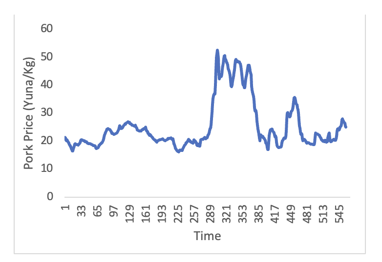
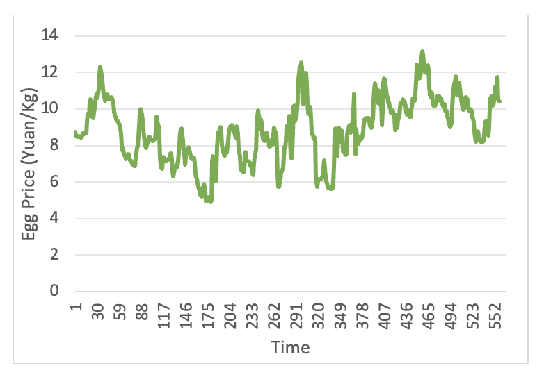
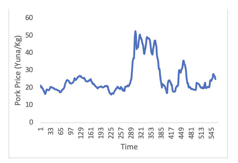
To further enhance the accuracy of the model and the availability and reliability of weekly data, this paper also considers the prices of shrimp substitutes, eggs, and pork. These data are sourced from the Agricultural Product Price Monitoring website of the Ministry of Agriculture of the People’s Republic of China (https://pfsc.agri.cn). By incorporating the price trends of these substitutes into the model, a more comprehensive understanding of the dynamics of shrimp prices can be gained, thereby improving the accuracy of the forecasts. The price trends of eggs and pork are shown in Figures 3 and 4. The volatility trend of pork prices from 2016 to 2022 is large, characterized by non-linearity and non-stationarity, while egg prices generally show a cyclical pattern of change.

Figure 3.Average weekly price trend of pork

Figure 4.Average Weekly Price Trend for Eggs

3.2. WOA-VMD Results

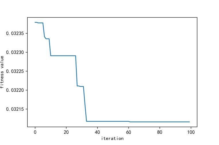
Among the VMD parameters, the number of fixed modes k is crucial for the realization of high prediction accuracy,²⁴ and to further improve the data quality and eliminate the influence of noise, WOA-VMD is used in this study to decompose the price series. First, the number of whales is set to 5, the maximum number of iterations is 100, the number of variables is 2, the penalty factor is [100,2000], the range of k values is [2,10], and only integers are included. Then, the optimal penalty parameter obtained by optimizing the VMD parameters using WOA is 960 and the optimal parameter for the intrinsic modal function (IMF) is 9.

Figure 5.results of whale optimization algorithm

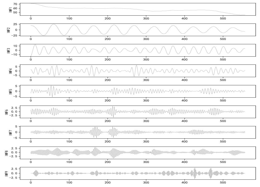
As can be seen in Figure 5, the whale algorithm gradually stabilizes after iterations, and Figure 6 demonstrates the results of the weekly average shrimp price data processed by the Variable Modal Decomposition (VMD).

Figure 6.Variational Modal Decomposition results

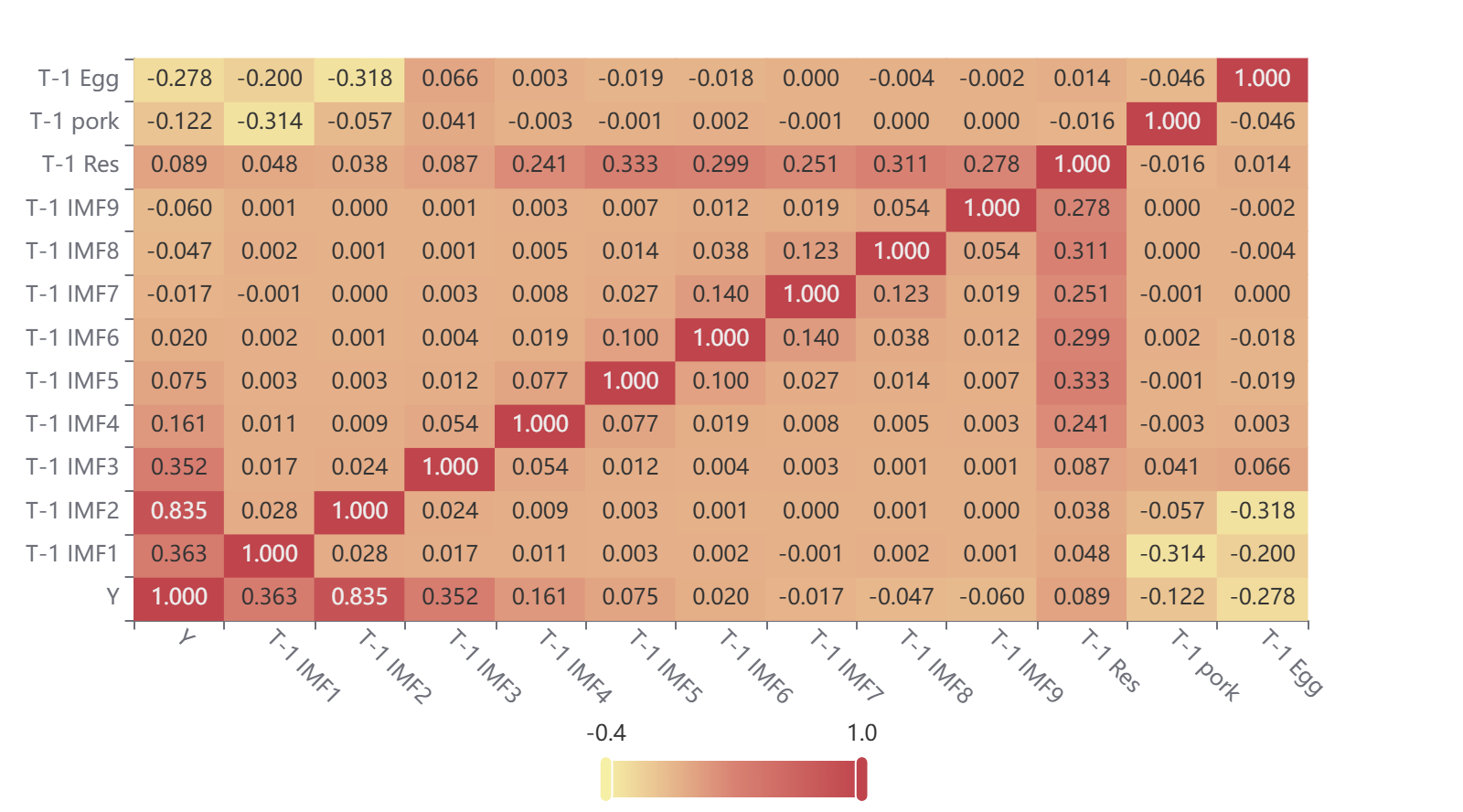
The Pearson’s correlation coefficients between the input variables and shrimp prices with one period lag are shown in Figure 7. Starting from the 4th IMF series, the Pearson correlation coefficient becomes smaller; combined with the above analysis, IMF1 is the trend term of the shrimp price time series, IMF2 is the cyclical term, IMF3 is the low-frequency term, and IMF4-9 is the high-frequency terms. The trend and cyclical terms are the main components of shrimp prices, reflecting the inherent long-term trend of shrimp prices; the low-frequency term has a wide range of fluctuations, representing the impact of major events on shrimp prices; the high-frequency term’s mean fluctuates up and down in the neighborhood of [-5,5], representing the short-term market imbalance in supply and demand and the price changes caused by unscheduled events.

Figure 7.Pearson correlation coefficient

3.3. Model Predictive Performance Analysis

In this paper, we analyzed the raw data of the weekly average price of shrimp by constructing three machine learning models: decision tree, AdaBoost, and XGBoost. To verify the predictive ability of the models, we divided 20% of the data samples into a test set and the remaining 80% as a training set. In the model inputs, we used feature variables lagged by one period. To ensure the reproducibility of the experiments, we set the number of random seeds to 291 when dividing the data. During model training, we used the default hyperparameters of the Sklearn library and set the random number seed to 1 before training to ensure that the test set produces more consistent results across experiments. In addition, we ensured the consistency of parameters such as evaluation metrics, training batch, learning rate, and training period. The prediction performance of the benchmark model is detailed in Table 1.

The mean absolute percentage error (MAPE) and the coefficient of determination (R²) are two key metrics when evaluating the performance of a model. The lower the MAPE value, the lower the prediction error; and the closer the R² value is to 1, the higher the model’s explanatory power. This study compares three machine learning models: decision tree, AdaBoost regression, and XGBoost. the results show that the R² value of the decision tree model is 0.771, which is the lowest among the three models; while the R² value of the XGBoost model is 0.864, which is the best performance. In addition, the MAPE value of the XGBoost regression prediction algorithm is 0.06, indicating that its prediction error is relatively small.Given the superior performance demonstrated by the XGBoost model in shrimp weekly average price forecasting, we chose the XGBoost model and combined it with the SHAP (SHapley Additive exPlanations) model for an in-depth analysis of the key factors affecting shrimp prices.

To avoid the overfitting problem of the XGBoost model, we need to optimize the model parameters. Bayesian optimization is a global optimization algorithm proposed by Pelikan et al²⁵ to find the optimal solution in high-dimensional non-convex search space to minimize the objective function, which uses Bayes’ theorem to construct an agent model and determines the next optimization scheme by continuously updating this agent model, and its convergence theory better guarantees the hyper-parametric approach to optimize the model.²⁶

In XGBoost hyperparameter tuning, Bayesian optimization automatically finds the best hyperparameter configurations to minimize model validation errors. In this paper, we identify the most important parameters and value ranges that may affect the validity of the XGBoost model. These parameters and value ranges will be replaced in the Bayesian optimization algorithm. The combinations of hyperparameters used for XGBoost model prediction are as follows: the optimal range of n_estimators is [10, 500]; the optimal range of max_depth is [1, 15]; and the optimal range of learning_rate is [0.01, 1]. The specific parameters are shown in Table 2.

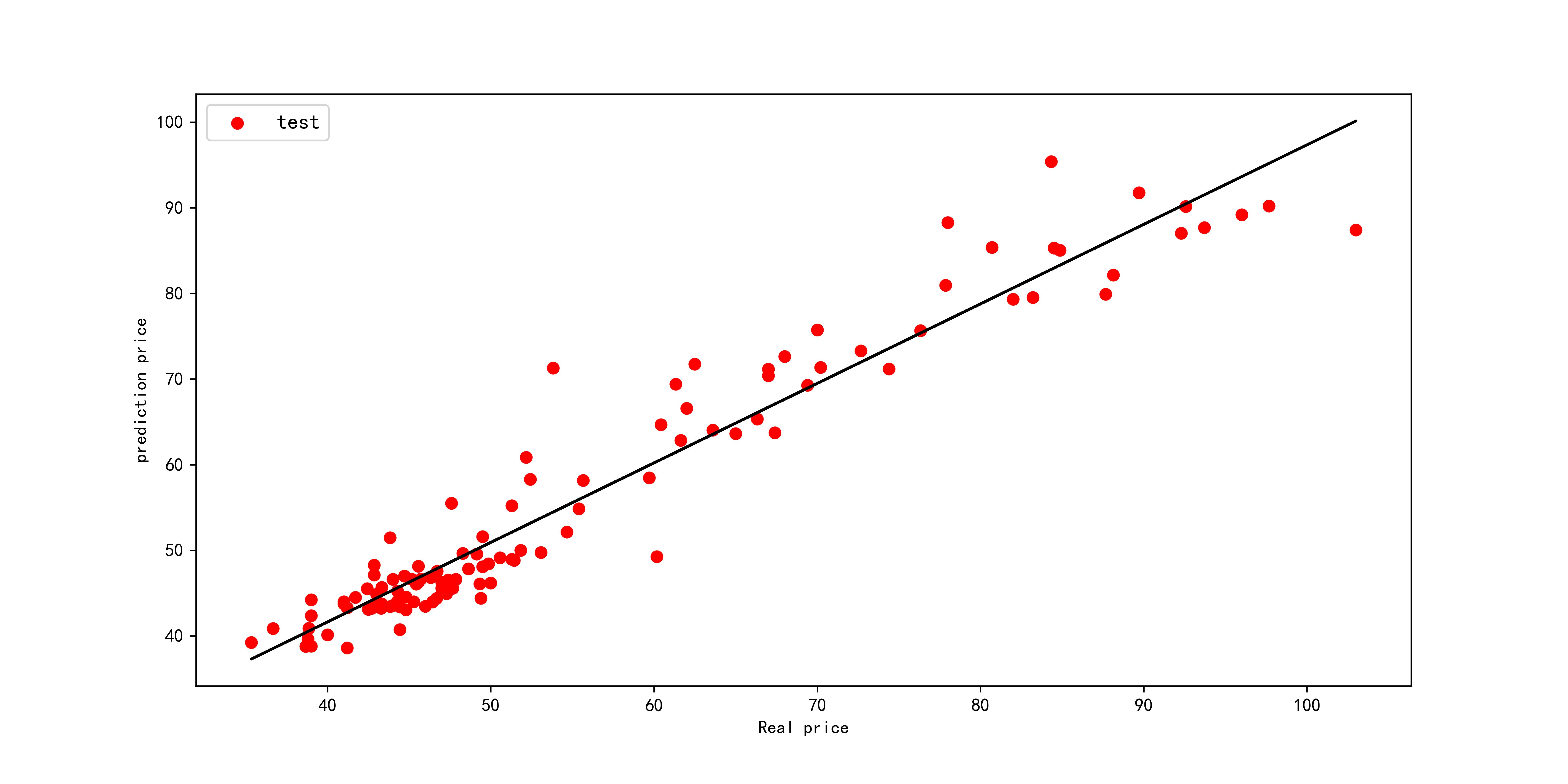
The RMSE, R², MAE, and MAPE of the BO-XGBoost prediction set are 4.36, 0.927, 3.08, and 0.05, respectively, which are better than the three benchmark models. The R² of the Bayesian-optimized XGBoost model improves by 4.98% over the benchmark XGBoost prediction model. In addition, we plotted the intersection of the scatters of the true and predicted values. Figure 8 shows that the scatters of the BO-XGBoost model are almost always clustered around the y=x line, indicating high prediction accuracy.

Figure 8.Bo-XGBoost model fitting for shrimp prediction

3.4. Model robustness analysis

3.4.1. K-fold cross-validation

This paper adopts the K-fold cross-validation method. The data set is divided into K copies, each time one of them as a test set, the remaining K-1 copies as a training set, repeated k times,²⁷ and finally, the average of the k times of the assessment index as the performance index of the constructed shrimp price weekly average price prediction model. In this paper, we choose 10-fold cross-validation; ten-fold cross-validation is a more stringent requirement for the stability and accuracy of the model; 10-fold cross-validation results are shown in Table 3.

Table 3 shows that the average R² of the training set and test set of the ten-fold cross-validation of the BO-XGBoost prediction model are 0.971 and 0.93, respectively, indicating that the model has excellent prediction performance and robustness.

3.4.2. Learning Curve

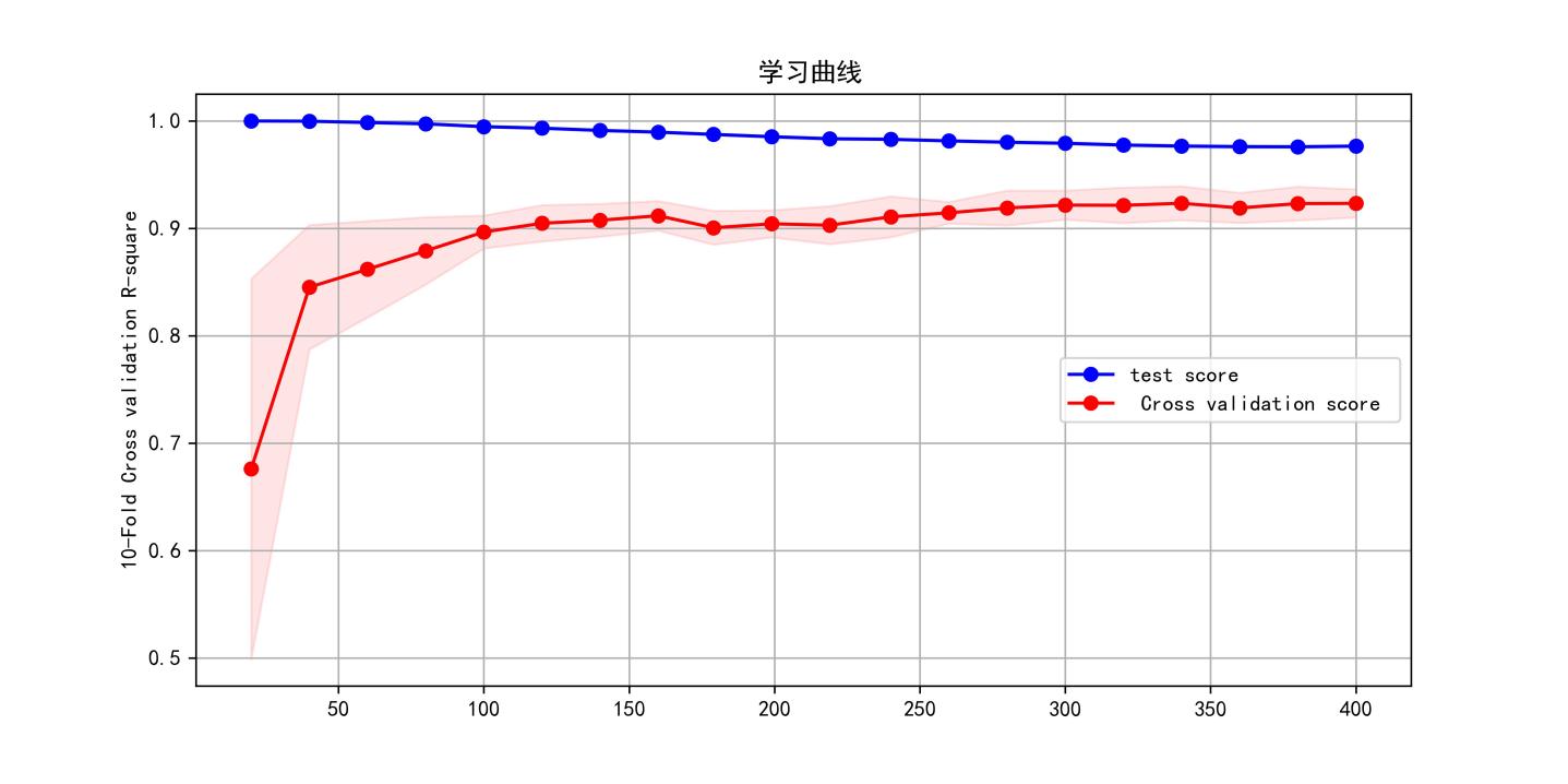
In addition, using the learning curve approach, we can plot the trend of the training error and test error concerning the dataset size, a common tool in machine learning to assess whether a model is overfitting or underfitting. When there is a significant gap between the training error and the test error, it may mean that the model is suffering from overfitting or underfitting. On the contrary, if the gap between the training error and the test error is small and gradually converges as the dataset size increases, the model has a good fitting performance. The learning curve is shown in Figure 9, from which it can be seen that as the number of samples increases, the difference between the R² of the training set and the test set of the Bo-XGBoost model gradually decreases and then converges to a single value, and there is no underfitting or overfitting in the BO-XGBoost model.

Figure 9.BO-XGBoost model learning curve

3.4.3. Detection of different datasets

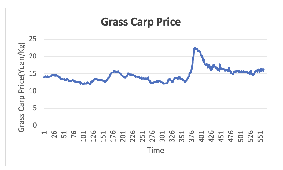
In order to verify the accuracy of the model’s prediction on other aquatic products data sets, the price data of grass carp, a common aquatic product, is selected for prediction, with the same data sources as in section 3.1, and the time range of the data set is taken as the daily price of agricultural products from January 1, 2014, to September 30, 2024, as shown in Figure 10. The forecasting methodology is the same as that in Section 3.3, and the three benchmark models are utilized to forecast the average weekly price of grass carp and the results of the model forecasts are shown in Table 4.

Figure 10.Trends in average weekly prices of grass carp

As can be seen from Table 4, the grass carp price prediction model based on XGBoost algorithm outperforms other benchmark models, and the RMSE、R²、MAE、and MAPE of the optimal model of its test set are 0.279, 0.982, 0.18, and 0.012, respectively, which indicates the applicability of the article’s VMD-XGBoost model to price prediction of different aquatic products.

3.5. SHAP model Analysis

Figure 11 shows the SHAP global feature analysis of the XGBoost model. The periodic term (IMF2) is the most important predictor of shrimp price. To explore the influence of features on the model output more intuitively and extract valuable information to help relevant government departments and enterprises take targeted measures, this paper adopts SHAP value mapping diagrams to show the nonlinear relationship between variables.²⁸ Unlike the partial dependency plot, the vertical coordinate of the SHAP value mapping plot is the SHAP value instead of the output label value,²⁹ which can effectively analyze the nonlinear effects of the important predictors affecting the fluctuation of shrimp prices.

Figure 11.SHAP Summary Plot

As shown in Figure 12, when the cyclical term represented by T-1 IMF2 is greater than 0, SHAP is positive and significantly affects prices, indicating that prices are beginning to enter an upward cycle.

Figure 12.Analysis of SHAP feature dependency plot

In the XGBoost model, feature importance reflects how much each predictor contributes to the model prediction. The higher the gain value of a feature, the higher the importance of that feature in the model prediction.

As Table 5 shows, the volatility of shrimp prices in Jiangsu Province is mainly affected by the cyclical term, and the characteristic importance of the cyclical term accounts for 67%. Compared with the SHAP summary plot, the feature rankings are basically the same, indicating the robustness of the feature importance rankings generated by the XGBoost model.

4. Conclusions

Fishery is one of the important industries in China, and its development is of great significance to the sustainable development of China’s economy and society and to guarantee China’s food security. The study shows that the WOA-VMD-XGBoost model optimized by Bayesian algorithm has a better predictive performance with R² of 0.927, which is better than the benchmark model. Visual analysis of the results of the SHAP interpretable tool shows that seasonal factors mainly influence shrimp price fluctuations and the characteristic importance of the cyclical term accounts for 67% of the total. It is difficult to make absolutely accurate forecasts of fish prices because they are affected by various factors. Further exploration and continuous efforts are needed to predict aquatic product prices more accurately.

For future research, more attention can be paid to the interpretable analysis of deep learning in the methodology, and the multimodal aquatic product price prediction model can be constructed by utilizing the Transformer framework. The application of methods such as unsupervised clustering and signal decomposition in identifying and predicting inflection points in the long-term trend cycle of aquatic product prices can be strengthened. In addition, early warning studies on specific aquatic product prices can be conducted based on the analysis results of various interpretable models such as SHAP and Lime. With regard to the many factors affecting fish prices, strengthen the use of satellite remote sensing to obtain more accurate meteorological data, finely account for production and processing costs, such as nursery quantities, fishmeal prices, aquaculture profits, and other key influencing factors, and utilize modern information technology means such as the Internet of Things, big data analysis and other modern information technology mean to collect and update fish price data in real-time and strive to dig into the laws reflected in the statistical monitoring data to improve the early-warning accuracy and effectiveness and strengthen risk tracking. At the level of forecasting model application, it strengthens the combination of federal learning and Web forecasting program, builds XGBoost security tree model, enhances privacy computing capability, and solves the problem of enterprise data availability.

Authors’ Contribution

Conceptualization: Zhan Wu (Lead). Methodology: Zhan Wu (Lead). Formal Analysis: Zhan Wu (Equal), Tinghong Qu (Equal). Writing – original draft: Zhan Wu (Lead). Supervision: Tinghong Qu (Lead). Writing – review & editing: Zongfeng Zou (Equal).

CONFLICT OF INTEREST

The authors declare that they have no conflicts of interest.

Funding

The author(s) received no financial support for this article’s research, authorship, and/or publication.

Data Availability Statement

The data supporting this study’s findings are available from the corresponding author upon reasonable request.

Informed Consent Statement

All authors and institutions have confirmed this manuscript for publication.