An Improved Active Disturbance Rejection Control Method for a Deep-Sea Aquaculture Vessel

undefined

Introduction

With the rapid advancement of technology and the increasing scarcity of resources, there is a growing need to explore the ocean for more resources. However, the deep-sea regions, which are rich in marine resources, present extremely complex environmental conditions. Engineering equipment operating in these deep-sea areas can be affected by factors such as wind, waves, and currents, causing them to deviate from their intended operational positions and trajectories. The application of Dynamic Positioning (DP) systems effectively mitigates these issues. DP systems were first introduced in the 1960s for maritime applications and have undergone three stages of development: initially, controllers based on classical control theory combining PID and low-pass filters were designed; subsequently, controllers were developed using modern control theory and Kalman filtering; and currently, intelligent control methods have been introduced, significantly enhancing the precision of DP controllers.

The design of DP controllers is the core of DP systems, playing a crucial intermediary role and serving as a primary standard for evaluating the development of DP systems. Among these, the control strategy algorithms in controller design are a major focus of research and a significant direction for improving dynamic positioning performance. Currently, the main control strategy algorithms include: PID control algorithm, Fuzzy Control algorithm, Backstepping Integral Control algorithm, Nonlinear Model Predictive Control algorithm, Fault-Tolerant Control algorithm, Neural Network algorithm, and Adaptive Combined Control methods.¹ Many of these control algorithms, such as Model Predictive Control (MPC) and fault-tolerant control, heavily rely on accurate mathematical models of the vessel to achieve effective control, which significantly reduces the generalizability of these methods.² In contrast, fuzzy logic control algorithms do not require precise models of the controlled object; however, their design necessitates extensive expert experience,³ which undoubtedly increases the complexity and cost of the design process and makes it challenging to cope with random disturbances. To more effectively study the application of dynamic positioning (DP) systems in ship control, it is essential to develop more control algorithms to address various scenarios.

In recent years, Active Disturbance Rejection Control (ADRC), which combines the advantages of simple structural design, ease of implementation, and independence from precise models of the controlled object, has garnered extensive attention from researchers in the control field and achieved significant progress. ADRC was first improved by Han Jingqing in 1998 based on PID control.⁴ Subsequently, more researchers in related fields have conducted in-depth studies and improvements on ADRC. ADRC was proposed to address nonlinear system problems. Zheng and Gao⁵ first linearized the nonlinear issues in ADRC systems, effectively reducing computational complexity. Humaidi and Badir⁶ compared the performance of NLADRC and LADRC, finding that the former exhibited superior dynamic performance while the latter showed stronger robustness.⁷ JianXin et al.⁸ incorporated an improved dragonfly algorithm into the IADRC system and applied it to fast steering mirrors (FSM), ultimately validating the control law’s achievement of high tracking accuracy in FSM. Y.E. et al.⁹ studied the principles of ADRC and compared it with PID control, analyzing their respective advantages and disadvantages, and then applied ADRC to DP systems. He-Jin et al.¹⁰ experimentally verified that ADRC outperformed PID control under strong disturbances. Chen et al.¹¹ improved the nonlinear FAL function in the ESO (Extended State Observer) of ADRC, enhancing its disturbance rejection performance, but also making parameter tuning more difficult. Yang et al.¹² combined the advantages of linear and nonlinear ADRC strategies, integrating a switching strategy that enabled switching between nonlinear and linear control, and applied this scheme to ship DP systems, though the switching conditions and strategy were not mature. Wu et al.¹³ improved the nonlinear ADRC using an artificial bee colony algorithm, effectively optimizing complex parameters but facing issues with optimization efficiency and difficulty in achieving optimal results. Wang et al.¹⁴ designed an adaptive weighted hybrid particle swarm algorithm to optimize the ADRC controller to handle model uncertainties in nonlinear ADRC systems, and introduced a cloud model intelligent algorithm into ship DP systems.¹⁵ Li¹⁶ et al. proposed a novel control strategy that employs a Long Short-Term Memory neural network to predict the heave motion of vessels and utilizes a Bayesian algorithm for hyperparameter optimization. Concurrently, the strategy incorporates a Chaotic Particle Swarm Optimization algorithm for the parameter tuning of Active Disturbance Rejection Control. This approach has been shown to significantly enhance the compensation accuracy and response speed of the Active Heave Compensation system.

In summary, current research on Active Disturbance Rejection Control (ADRC) primarily focuses on addressing the control accuracy and computational complexity of nonlinear control systems. However, there is insufficient research on the numerous parameters of ADRC and the difficulty of tuning them, which makes it challenging to achieve both strong disturbance rejection and effective parameter tuning simultaneously. Presently, research on control systems for deep-sea aquaculture workboats, as an emerging aquaculture system, is lacking, making it difficult to cope with the strong disturbances in the deep-sea aquaculture environment. To address these shortcomings, this study takes aquaculture workboats as the research object, designing a dynamic positioning controller based on an improved ADRC strategy for deep-sea aquaculture workboats. The controller’s parameters are optimized and tuned using an improved Whale Optimization Algorithm. The goal is to ensure that the dynamic positioning system has strong disturbance rejection capabilities and rapid, effective dynamic control, thereby enhancing the safety of marine aquaculture equipment, improving operational efficiency, and promoting the development of marine engineering towards deep-sea operations. This has practical significance for the transition of marine engineering equipment towards automated and intelligent management.

Materials and Methods

1.DP system is applied to the frame design of deep-sea aquaculture vessels

The deep-sea aquaculture vessel is a farming system based on a ship platform, capable of either drifting or stationary farming at sea according to demand. It effectively enhances the quality of aquatic products in deep-sea fishery farming, addresses the scarcity of coastal space resources and the insufficiency of water resources, reduces water pollution or eutrophication, and significantly mitigates the limitations and unsustainability of traditional aquaculture. This represents a novel direction in deep-sea aquaculture.

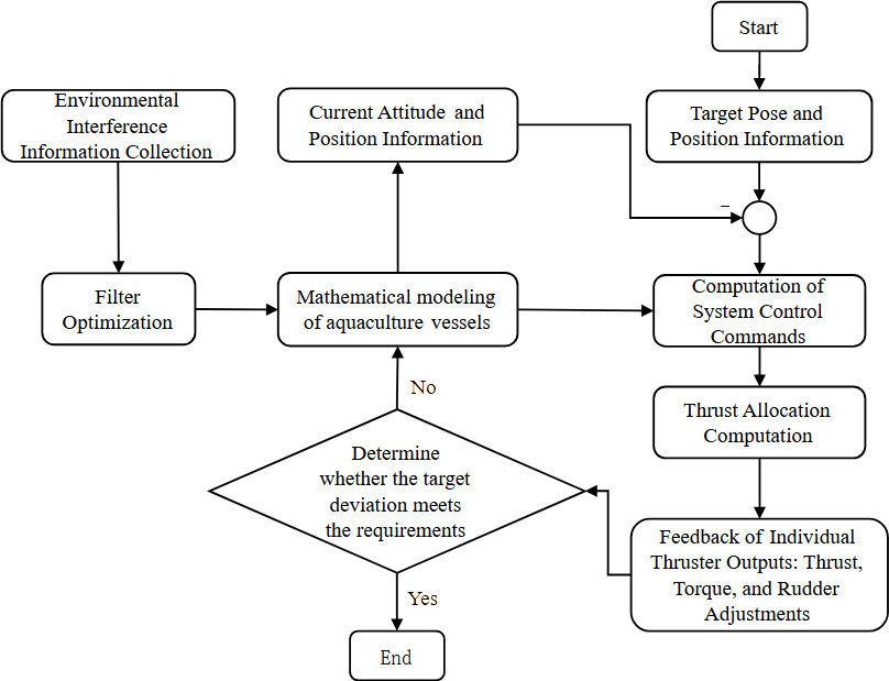
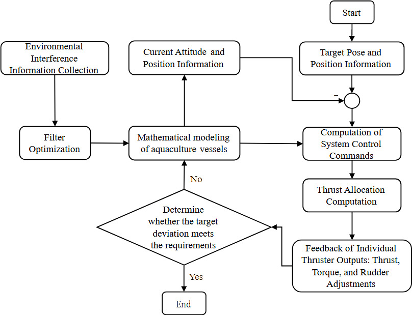
The application of a Dynamic Positioning (DP) system on deep-sea aquaculture vessels enables motion control in the horizontal plane, thereby ensuring stable positioning of the vessel in the marine environment. This stability is crucial for maintaining a secure farming environment. Deep-sea aquaculture vessels are subject to dynamic disturbances from external environments such as wind, waves, and currents, as well as hydrodynamic coupling disturbances from the internal aquaculture tank’s liquid level. These disturbances are variable, making it difficult to establish precise mathematical motion models. ADRC can integrate the unknown disturbances and other uncertainties of the system into a total disturbance, which is then compensated by the Extended State Observer (ESO), ultimately achieving control over the system with time-varying uncertainties.¹⁷ Based on this, this study utilizes the ADRC strategy to design a controller for the dynamic positioning system of deep-sea aquaculture workboats under irregular external environmental disturbances and coupling effects among the vessel’s degrees of freedom.

The application technical scheme flow of the DP system is illustrated in Figure 1.

2. Mathematical model of ship motion

2.1. Kinematic equations

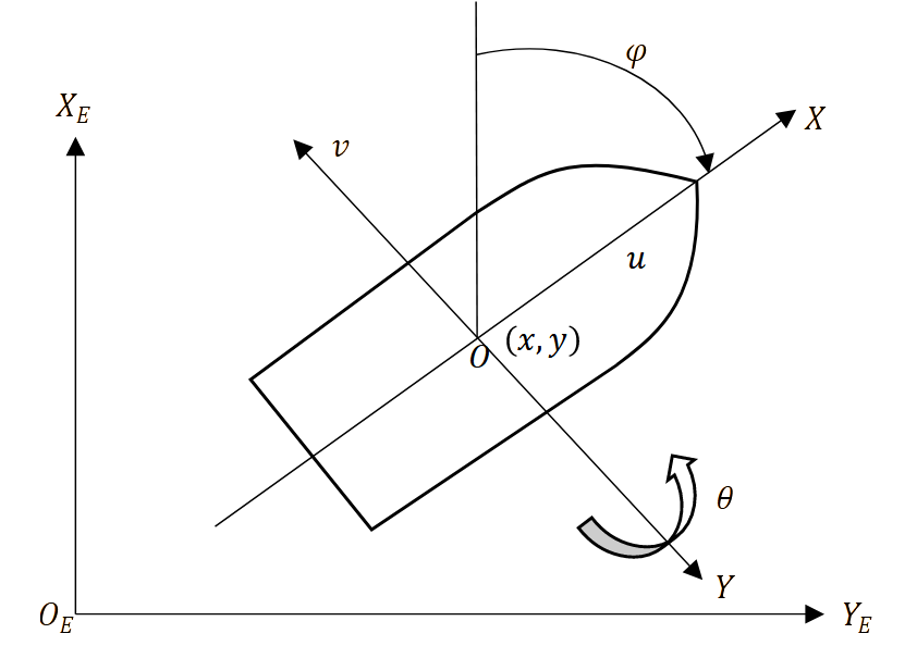
On the sea surface, due to the combined effects of wind, waves, and currents, a ship’s motion manifests as six degrees of freedom without constraints. However, the roll and pitch angles of the ship are generally small and do not affect the ship’s displacement significantly, so the ship’s motion is often simplified to three degrees of freedom. Two coordinate systems are commonly used for ship motion modeling: the North-East coordinate system ($X_{E}O_{E}Y_{E}$) and the ship-fixed coordinate system (XOY). As shown in Figure 2. The vertical axis Z of both coordinate systems points vertically toward the center of the Earth.³

For the simplified expression of three degrees of freedom (surge, sway, yaw), the longitudinal position, lateral position, and heading angle of the ship in the North-East coordinate system can be defined as the vector $\mathbf{\eta} = \lbrack x，y，\psi\rbrack^{T}$, and the longitudinal velocity, lateral velocity, and yaw rate of the ship in the ship-fixed coordinate system can be defined as the vector $\mathbf{\upsilon} = \lbrack u，v，r\rbrack^{T}$. The transformation matrix between these two coordinate systems is denoted as $\Upsilon(\psi)$, and satisfies $\Upsilon^{- 1}(\psi) = \Upsilon^{T}(\psi)$. The transformation matrix and the transformation relationship are given by equations (1) and (2)¹⁸:

$$\begin{array}{r} \Upsilon(\psi) = \begin{bmatrix} cos\psi & - sin\psi & 0 \\ sin\psi & cos\psi & 0 \\ 0 & 0 & 1 \end{bmatrix}\tag{1} \end{array}$$

$$\begin{array}{r} \dot{\mathbf{\eta}} = \Upsilon(\psi)\mathbf{\upsilon}\tag{2} \end{array}$$

In the above equations, $\psi$ represents the yaw angle, $\mathbf{\eta}$ is the vector of position and attitude information defined in the North-East coordinate system as $\lbrack x，y，\psi\rbrack^{T}$, $\mathbf{\upsilon}$ is the vector of velocity information defined in the ship-fixed coordinate system as $\lbrack u，v，r\rbrack^{T}$.

2.2. Ship low frequency motion model

In ship motion, high-frequency movements do not affect the displacement of the hull. Therefore, only the low-frequency nonlinear motion model of the vessel is considered, as shown in Equation (3).^3,18

$$\begin{array}{r} M\dot{v} + Dv = \Upsilon^{T}(\psi)b + \tau\tag{3} \end{array}$$

In equation (3), M is the system inertia matrix including additional mass effects as shown in equation (4), and D is the hydrodynamic damping coefficient matrix as shown in equation (5), both of which are positive definite. τ represents the output control force and moment, and b represents environmental disturbance forces and moments such as wind, waves, and second-order drift. These disturbances are typically considered to affect slow movements and are represented as shown in equation (6).

$$\begin{array}{r} M = \begin{bmatrix} m - X_{\dot{u}} & 0 & 0 \\ 0 & m - Y_{\dot{v}} & mx_{G} - Y_{\dot{r}} \\ 0 & mx_{G} - Y_{\dot{r}} & I_{z} - N_{\dot{r}} \end{bmatrix}\tag{4} \end{array}$$

In equation (4), $I_{z}$ is the moment of inertia about the Z axis, $X_{\dot{u}}$，$Y_{\dot{v}}$ and $N_{\dot{r}}$ are additional masses introduced by accelerations in the three degrees of freedom (surge, sway, yaw), and $Y_{\dot{r}}$ is the additional mass caused by the coupling of sway and yaw. $x_{G}$ is the distance from the ship’s center to the center of gravity.

$$\begin{array}{r} D = \begin{bmatrix}- X_{u} & 0 & 0 \\ 0 & - Y_{v} & - Y_{r} \\ 0 & - N_{v} & - N_{r} \end{bmatrix}\tag{5} \end{array}$$

$$\begin{array}{r} \dot{b} = - T^{- 1}b + E_{b}\omega_{b}\tag{6} \end{array}$$

In equation (5), $X_{u}$ represents the straight-line hydrodynamic damping coefficient, while $Y_{v}$, $Y_{r}$, $N_{v}$, and $N_{r}$ denote the linear hydrodynamic coefficients.

In equation (6), $T$ is a diagonal matrix of large time constants, the equation can be simplified as:

$$\begin{array}{r} \dot{b} = E_{b}\omega_{b}\tag{7} \end{array}$$

In equation (7), $E_{b}$ represents the noise amplitude, and is the coefficient matrix of zero-mean Gaussian white noise $\omega_{b}$.

Combining all the aforementioned descriptive equations, the linear state-space equation for the low-frequency motion of the ship is:

$$\begin{array}{r} \left\{ \begin{array}{r} {\dot{x}}_{L} = A_{L}x_{L} + B_{L}\tau + E_{L}\omega_{L} \\ y_{L} = C_{L}x_{L} + D_{L}\upsilon \end{array} \right. \tag{8} \end{array}$$

In equation (8), $x_{L}$ is the state variable, $y_{L}$ is the three-dimensional measurement position vector (yaw, surge, sway), $\omega_{L}$ is the three-dimensional unmodeled environmental disturbance variable, $\upsilon$ is the three-dimensional measurement Gaussian white noise; the matrix is defined as shown in equation (9)³:

$$\begin{array}{r} \left\{ \begin{array}{r} \ A_{L} = \begin{bmatrix} 0_{3 \times 3} & I_{3 \times 3} \\ 0_{3 \times 3} & - M^{- 1}D \end{bmatrix} \\ B_{L} = \begin{bmatrix} 0_{3 \times 3} \\ M^{- 1} \end{bmatrix} \\ E_{L} = \begin{bmatrix} 0_{3 \times 3} \\ M^{- 1} \end{bmatrix} \\ C_{L} = \begin{bmatrix} I_{3 \times 3} & 0_{3 \times 3} \end{bmatrix}, \end{array} \right.\ \tag{9} \end{array}$$

3.Design of automatic disturbance rejection controller for DP system

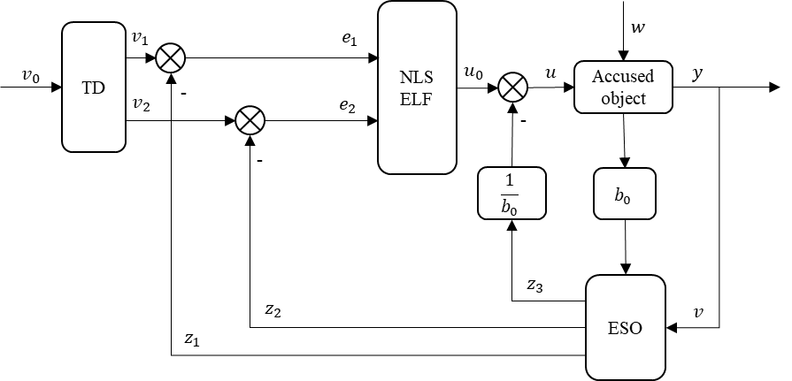
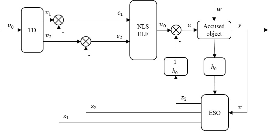
The paper takes a large-scale aquaculture support vessel as an example and proposes a DP control system based on the characteristics of its non-linear, multi-parameter unknown time-varying disturbances, and unstable model structure, with the core being the Active Disturbance Rejection Control (ADRC). The controller consists mainly of three parts: the Tracking Differentiator (TD), the Extended State Observer (ESO), and the Nonlinear State Error Feedback Control Law (NLSEF).⁵ The design process of the ADRC for dynamic positioning is formulated as follows:

1. Based on the characteristics of the deep-sea aquaculture support vessel, approximate mathematical modeling analysis is conducted. The core of this controller, the Extended State Observer (ESO), does not differentiate between internal and external disturbances of the system. It treats the internal and external disturbances as a whole, using a special feedback mechanism to make the observed value follow the actual value, without relying on the precise model of the controlled object.

2. According to the approximate mathematical model of the control system, the required controlled state variables are analyzed to determine the order of controller design.

3. Then, based on the control system’s order, design the core control parts corresponding to the controller, such as TD, ESO, etc. Then, according to the logical relationship, connect the established parts.

4. Finally, tune the relevant controller parameters. Due to the small coupling of each parameter, a separable method can be adopted to tune each part’s parameters one by one, and finally unify them in coordination.

The Active Disturbance Rejection Control (ADRC) structure is shown in Figure 3⁵.

3.1. Differential Tracker (TD)

Conventional differentiators amplify the noise input of the system, seriously affecting the system’s stability. The formula for the tracking differentiator used in this paper is:

$$\small \begin{array}{r} \left\{ \begin{array}{r} x_{1}(t + h) = x_{1}(t) + hx_{2}(t) \\ x_{2}(t + h) = x_{2}(t) + hfst\left( x_{1}(t) - v(t),x_{2}(t),r,h_{0} \right) \end{array} \right.\ \tag{10} \end{array}$$

In Equation (10), r is the velocity factor, determining the system’s tracking speed, h is the integration step size, $h_{0}$ is the filtering factor for filtering out noise. The definition of the optimal comprehensive function for fast control, $fst( \cdot )$ is as follows:

$$\begin{array}{r} \left\{ \begin{array}{r} d = rh \\ d_{0} = dh \\ y = x_{1} + hx_{2} \\ a_{0} = \sqrt{d^{2} + 8r|y|} \\ a = \left\{ \begin{array}{r} x_{2} + \frac{\left( (sgny)a_{0} + d \right)}{2},\ \ \ \ \ \ \ \ \ \ \ \ \ |y| > d_{0} \\ x_{2} + \frac{y}{h},\ \ \ \ \ \ \ \ \ \ \ \ \ \ \ \ \ \ \ \ \ \ \ \ \ \ \ \ \ \ \ \ \ \ \ \ \ |y| \leq d_{0} \end{array} \right.\ \\ fst = - \left\{ \begin{array}{r} \frac{ra}{d},\ \ \ \ \ \ \ \ \ \ \ \ \ \ \ \ \ \ \ \ \ \ \ \ \ \ \ \ \ \ \ \ \ \ |a| \leq d \\ rsgn(a),\ \ \ \ \ \ \ \ \ \ \ \ \ \ \ \ \ \ \ \ \ \ \ \ |a| > d \end{array} \right.\ \end{array} \right.\ \tag{11} \end{array}$$

The final form of the TD arrangement transition process is:

$$\small \begin{array}{r} \left\{ \begin{array}{r} v_{1}(k + 1) = v_{1}(k) + hv_{2}(k) \\ v_{2}(k + 1) = v_{2}(k) + hfst\left( v_{1}(k) - v_{0},v_{2}(k),r,h_{0} \right) \end{array} \right.\ \tag{12} \end{array}$$

Among them, $v_{0}$ is the setting value.

3.2. Expanded State Observer (ESO)

The dynamic positioning system is a discrete-time control system, and its application scenario can be considered as a second-order system. The role of the Extended State Observer (ESO) is to treat the internal and external disturbances of the system as a whole and suppress their disturbances using nonlinear feedback effects. Therefore, the discrete forms of its state estimation and total disturbance equations are as follows¹⁹:

$$\small \begin{array}{r} \left\{ \begin{array}{r} \varepsilon_{1} = z_{1}(k) - y(k) \\ z_{1}(k + 1) = z_{1}(k) + h\left( z_{2}(k) - \beta_{01}\varepsilon_{1} \right) \\ z_{2}(k + 1) = z_{2}(k) + h\left( z_{3}(k) - \beta_{02}fal\left( \varepsilon_{1},\alpha_{1},\delta \right) + bu(k) \right) \\ z_{3}(k + 1) = z_{3}(k) - {h\beta}_{03}fal\left( \varepsilon_{1},\alpha_{2},\delta \right) \end{array} \right.\ \tag{13} \end{array}$$

In Equation (13), $\varepsilon_{1}$ represents the system error; $0 < \alpha_{2} < \alpha_{1} < 1$ are empirical values, and for the sake of analogy, we set the proportional-like gain $\alpha_{1} = 0.5$ and the differential gain $\alpha_{2} = 0.25$, $\beta_{01},\ \ \beta_{02},\ \ \beta_{03}$ are the adjustable gain coefficients, all greater than 0, b is the compensation factor. The fal function used has the characteristics of small error and large gain, as well as large error and small gain, as shown in Equation (14):

$$\begin{array}{r} fal(\varepsilon,\alpha,\delta) = \left\{ \begin{array}{r} |\varepsilon|^{\alpha}sgn(\varepsilon)，\ \ \ \ \ \ |\varepsilon| > \delta \\ \frac{\varepsilon}{\delta^{1 - \alpha}}，\ \ \ \ \ \ \ \ \ \ \ \ \ |\varepsilon| \leq \delta \end{array} \right.\ ，\delta > 0 \tag{14} \end{array}$$

where $\varepsilon$ represents the input error.

3.3. Nonlinear state error feedback control law (NLSELF)

The calculation of the control law includes two parts: (1) Compensation for the tracking signal error and the differential signal error (analogous to PD control); (2) Compensation for disturbance rejection. The classical PID controller calculates the proportional, integral, and derivative controls as a weighted sum, which has a major drawback of parameter coupling. This coupling makes tuning difficult and may prevent achieving the optimal combination. This paper uses a “nonlinear combination” approach to effectively address this issue.

NLSELF is given by equation (15)²⁰:

$$\scriptsize \begin{array}{r} \left\{ \begin{array}{r} e_{1} = v_{1}(k) - z_{1}(k) \\ e_{2} = v_{2}(k) - z_{2}(k) \\ e_{3} = \int_{\mathstrut}^{\mathstrut}{e_{1}dt} \\ u_{0} = \beta_{1}fal\left( e_{1},\alpha_{1},\delta_{1} \right) + \beta_{2}fal\left( e_{2},\alpha_{2},\delta_{2} \right) + \beta_{3}fal\left( e_{3},\alpha_{3},\delta_{3} \right) \\ u(k) = u_{0} - \frac{z_{3}(k)}{b_{0}} \end{array} \right.\ \tag{15} \end{array}$$

Among them, $e_{1}$, $e_{2}$, $e_{3}$ represents the state error, $\beta_{1}$, $\beta_{2}$ and $\beta_{3}$ represent the feedback control gains, $\alpha_{3}$ is a proportional-like integral gain, with $- 1 < \alpha_{3} < 1$, $u_{0}$ represents the extracted nonlinear combination signal $z_{3}$ is the disturbance estimate output by ESO, and $\frac{z_{3}(k)}{b_{0}}$ is defined as the disturbance compensation amount, which compensates for the initial control quantity, $u(k)$ is the final control output of ADRC.

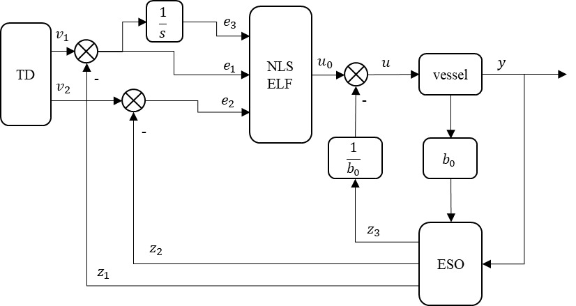
3.4. Improved automatic disturbance rejection control design

Traditional ADRC systems based on PID control combine the proportional and derivative gain coefficients into an NLSELF gain parameter. This paper considers adding an integral gain parameter to optimize the NLSELF combination with analogous proportional, derivative, and integral gain coefficients. The Improved Active Disturbance Rejection Control (IADRC) system is shown in Figure 4.

To verify the effectiveness of the IADRC control system, a second-order system $\frac{s + 4}{s^{2} + 4s + 6}$ will be used as the controlled object for position tracking simulation. The results are shown in Figure 5.

The introduction of an integral component to the traditional ADRC structure enhances the system by incorporating additional state error variables and a novel error feedback control gain. This modification enriches the diversity and superiority of nonlinear error feedback control law configurations, thereby improving system control precision. As shown in Figure 5, the designed IADRC controller demonstrates good control tracking performance. However, a drawback is the difficulty in parameter tuning. Therefore, an optimization algorithm for tuning the parameters of the active disturbance rejection controller will be introduced in the following section.

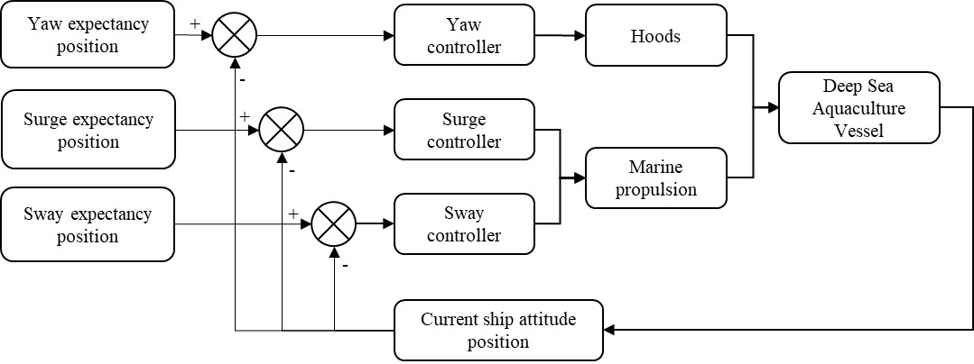
3.5. Design of DP active disturbance rejection control system

Referring to the separability concept and analyzing the mathematical model of motion for the deep-sea aquaculture support vessel, it can be understood that the control of the ship in the three degrees of freedom (heave, sway, and yaw) can be conducted independently. Due to the fact that the ADRC does not differentiate between internal and external disturbances, the coupling effects among these three degrees of freedom are treated as overall disturbances and compensated for. Therefore, this paper will design three different controllers to control the heave, sway, and yaw degrees of freedom respectively. By comparing the desired positions and current positions in the three degrees of freedom directions, as well as the desired yaw angle and current yaw angle, the deviation inputs to the controllers are obtained. The controllers calculate and output the control quantities in each degree of freedom direction. The DP control structure diagram is shown in Figure 6.

4. Improved whale optimization algorithm

The Active Disturbance Rejection Controller (ADRC) is complex, with many parameters, most of which are adjustable and typically manually tuned. These parameters remain constant throughout the system operation and do not change. However, in practical engineering applications, the controlled objects and external disturbances are continuously changing. Without sufficient prior experience, it is difficult to determine the optimal coefficient gains and combination optimizations required by the controller to meet the desired performance. The Whale Optimization Algorithm (WOA) is a metaheuristic optimization algorithm designed to mimic the hunting process of humpback whales. It has a simple overall process, an easy-to-implement structure, requires few tuning parameters, and is well-suited for optimizing system parameters. In this section, an improvement is made to the WOA, and the Improved Whale Algorithm (IWOA) is used to optimize the parameters that have a significant impact on the ADRC.

4.1. Principle of whale optimization algorithm

This method consists of three main stages: encircling the prey, bubble-net feeding, and searching for prey. Each whale individual’s position represents a potential solution, which continuously iterates in the solution space to update the individual’s optimal position, ultimately leading to the acquisition of the global optimal solution.²¹

Typically, the initialization of a population is generated randomly, making it difficult to ensure the quality of the initial population. Therefore, this study considers the introduction of a nonlinear Skew Tent mapping model (as shown in Equation (16)),²² which has a more uniform probability density and faster iteration speed, to generate chaotic sequences for initialization.

$$\begin{array}{r} \left\{ \begin{array}{r} x_{k + 1} = \frac{x_{k}}{\varphi}，\ \ \ \ \ \ \ \ \ \ \ \ \ \ \ \ \ \ \ \ \ \ \ \ \ \ \ \ \ 0 < x_{k} < \varphi \\ x_{k + 1} = \frac{\left( 1 - x_{k} \right)}{(1 - \varphi)}，\ \ \ \ \ \varphi < x_{k} < 1 \end{array} \right.\ \tag{16} \end{array}$$

In equation (16), when $\varphi \in (0，1)$ and $x \in \lbrack 0，1\rbrack$, it represents a chaotic state.

1)Encircling Prey

Assuming the current best solution is the target optimal solution, after defining the best search method, other search agents will tend toward the best search agent and update their positions accordingly. This can be represented by the following equation (17):

$$\begin{array}{r} \left\{ \begin{array}{r} D_{1} = \left| CX^{*}(t) - X(t) \right| \\ X(t + 1) = X^{*}(t) - A \cdot D_{1} \end{array} \right.\ \tag{17} \end{array}$$

In the above equation, t represents the current iteration number, $X^{*}(t)$ is the vector of the best position up to now, $X(t)$ is the position vector of the current individual, $A$ and $C$ are coefficient vectors, represented as follows in equation (18):

$$\begin{array}{r} \left\{ \begin{array}{r} A = 2a \cdot r - a \\ C = 2 \cdot r \\ a = 2 - \frac{2t}{T_{\max}} \end{array} \right.\ \tag{18} \end{array}$$

In the above equation, $a$ decreases linearly from 2 to 0 over the whole process, while $r$ is the random vector in [0,1] and $T_{\max}$ is the maximum number of iterations.

To enhance the global search capability of WOA and avoid falling into local optima, this study incorporates an improved adaptive inertia weight ω into the process of updating individual positions as shown in equation (19).²³ In the early iterations, a larger ω can enhance global search, in the later iterations, a smaller ω should be used to facilitate local optimization.

$$\begin{array}{r} \left\{ \begin{array}{r} \omega = 1 + \sin\left( \frac{\pi t}{2t_{\max}} \right) \\ X(t + 1) = {\omega X}^{*}(t) - A \cdot D_{1} \end{array} \right.\ \tag{19} \end{array}$$

Where, $t$ represents the current iteration number, and $t_{\max}$ is the maximum number of iterations. The dynamic nonlinear nature of $\omega$ is used to control the extent to which the whale positions affect the positions of new individuals in the population.

Furthermore, by observing the WOA algorithm, it can be seen that the algorithm’s global search capability largely depends on the value of A. From equation (17) and (18), it is evident that A changes with a. Therefore, this paper adopts a nonlinear convergence factor a (as shown in equation (20)), which dynamically changes nonlinearly with the increase of the iteration number, to balance the global and local search capabilities of the WOA algorithm:

$$\begin{array}{r} a(t) = \left( a_{s} - a_{e} \right) - \left( \frac{\left( t_{\max} - t \right)}{t_{\max}} \right)^{m}\tag{20} \end{array}$$

Where, $a_{s}$ and $a_{e}$ represent the starting and ending values of the convergence factor, respectively $t$ is the current iteration number, $t_{\max}$ is the maximum number of iterations, $m \in (0，1)$ represents the nonlinear adjustment coefficient.

2)Bubble-net attack

When whales use bubble-net feeding, they move in a spiral shape between themselves and the prey. This can be imitated and expressed by the spiral equation as shown in equation (21):

$$\begin{array}{r} \left\{ \begin{array}{r} X(k + 1) = D^{\prime} \cdot e^{lb} \cdot \cos(2\pi l) + X^{*}(t) \\ D^{\prime} = \left| X^{*}(t) - X(t) \right| \end{array} \right.\ \tag{21} \end{array}$$

In the above formula, $D^{\prime}$ is the distance from the current search entity to the optimal solution; $b$ is the constant that defines the logarithmic spiral shape, and $l$ is the random number between [−1,1].

As humpback whales spiral closer to their prey, they move along two paths: a spiral path and a shrinking circle path. To simulate this behavior, during the optimization update, the spiral and circle shrinking paths are chosen based on a probability pp. The position update model is as follows in equation (22):

$$\small \begin{array}{r} X(k + 1) = \left\{ \begin{array}{r} {\omega X}^{*}(t) - A \cdot D_{1},\ p < 0.5 \\ D^{\prime} \cdot e^{lb} \cdot \cos(2\pi l) + X^{*}(t),\ p \geq 0.5 \end{array} \right.\ \tag{22} \end{array}$$

Where $p$ is the random number in [0,1].

3)Search for prey

To ensure that all whale individuals can fully search for prey, this optimization algorithm updates the positions based on the distances between each individual. When $|A| < 1$, the optimal search strategy is chosen for local search to update the position, as shown in equation (19), when $|A| > 1$, indicating a need to move away from the reference individual, a random search strategy is chosen for global search to implement the encircling mechanism. The equation is as follows in equation (23):

$$\begin{array}{r} \left\{ \begin{array}{r} D_{2} = \left| C \cdot X_{rand}(t) - X(t) \right| \\ X(t + 1) = {\omega X}_{rand}(t) - A \cdot D_{2} \end{array} \right.\ \tag{23} \end{array}$$

Where, $X_{rand}(t)$ is the position vector of random individuals in the current population.

The comprehensive search position update strategy is as follows:

$$\scriptsize \begin{array}{r} X(k + 1) = \left\{ \begin{array}{r} X^{*}(t) - A \cdot D_{1},\ p < 0.5 \cup |A| < 1 \\ D^{\prime} \cdot e^{lb} \cdot \cos(2\pi l) + X^{*}(t),\ p \geq 0.5 \cup |A| < 1 \\ X_{rand}(t) - A \cdot D_{2},\ p < 0.5 \cup |A| > 1 \end{array} \right.\ \tag{24} \end{array}$$

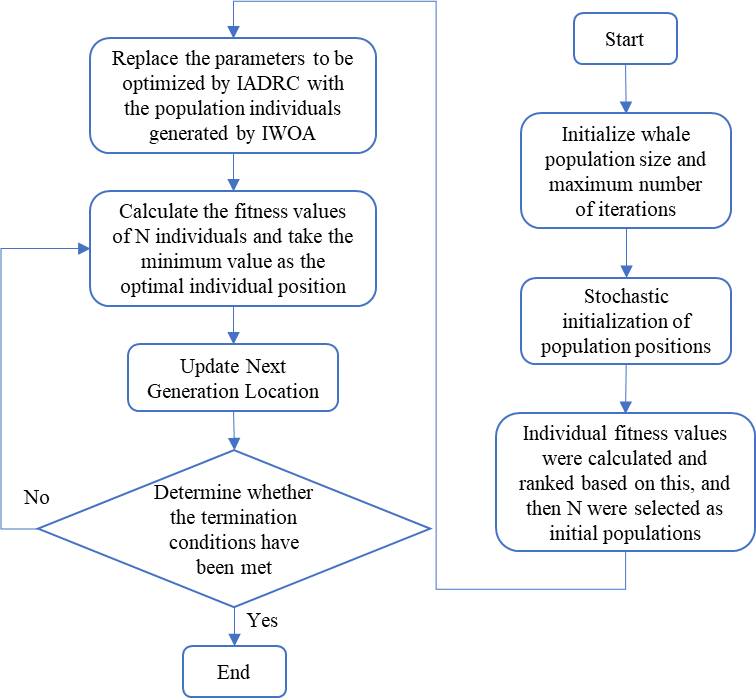
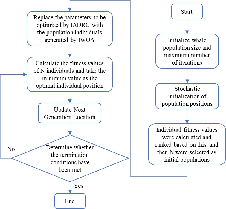
The IWOA algorithm flow is as follows:

Step 1: Define the population size, search space dimensionality, and maximum number of iterations. Initialize the whale population, individual positions, convergence factor a, and parameter vectors A and C.

Step 2: Calculate the fitness value of each individual in the whale population and select the top N individuals based on their fitness rankings.

Step 3: Replace the six tunable coefficients in the IADRC with the individuals generated by the IWOA.

Step 4: Update the positions of the individuals under the guidance of the six tunable coefficients.

Step 5: Update the convergence factor a and the parameter vectors A and C.

Step 6: Calculate the fitness values of the population individuals and update the positions of the six tunable coefficients in the IADRC.

Step 7: Determine whether the maximum number of iterations has been reached. If the maximum number of iterations has been reached, terminate the computation and output the optimal positions. If not, repeat Steps 2 to 6.

4.2. IWOA algorithm performance index test

In order to verify the effectiveness and advantages of the Improved Whale Optimization Algorithm (IWOA) proposed in this paper, it is compared with the Whale Optimization Algorithm (WOA), Genetic Algorithm (GA), and Grey Wolf Optimizer (GWO) using three test functions (as shown in Table 1). The population size is set to 30, and the number of iterations is set to 500. The final results of the three algorithms are recorded as shown in Table 2.

From Table 2, it can be observed that for the three test functions $f_{1}(x)$, $f_{2}(x)$ and $f_{4}(x)$, within 500 iterations, the experimental results show that the IWOA algorithm achieves significantly higher accuracy in terms of the optimal and average values compared to the other three algorithms. This makes it easier to obtain the optimal solution.

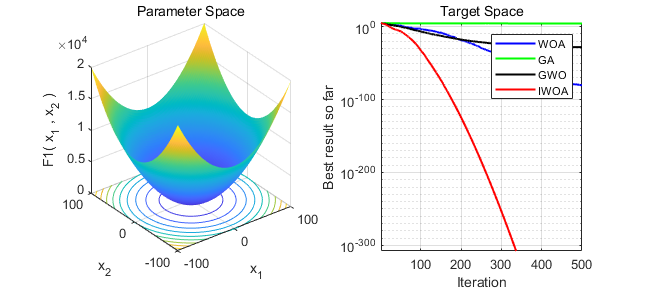
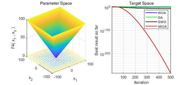
The convergence speeds of the four algorithms with a uniform number of iterations set to 500 are shown in Figure 7 to Figure 9.

Whereas, in Figure 7, the test function is $f_{1}(x)$, with a smooth surface in the function space on the left and the unique optimal solution at 0 on the bottom. The right side shows the target space graph, indicating that the IWOA algorithm reaches the optimal solution around iteration 340, demonstrating that the convergence speed and accuracy of the IWOA are significantly faster and better than the other three algorithms. In Figure 8, the test function is $f_{2}(x)$, which has several local optimal solutions and a global optimal solution in the function space. The graph on the right shows that the IWOA can reach the optimal solution at iteration 500, while the other three algorithms cannot converge to the optimal solution, indicating that the optimization speed and accuracy of the IWOA are superior to the other three algorithms. In Figure 9, the test function is $f_{4}(x)$, which has discontinuities in the function space. The graph on the right shows that the IWOA can find the optimal solution within 500 iterations, demonstrating the highest convergence speed and accuracy.

Hereby, It can be concluded that the Improved Whale Optimization Algorithm (IWOA) proposed in this paper optimizes the initial population to ensure its diversity and uniformity. During the position update process, an improved adaptive inertia weight ω is incorporated. Additionally, a nonlinear convergence factor a is introduced, which varies nonlinearly with the increase in iteration count to balance the algorithm’s global exploration and local exploitation capabilities. The algorithm exhibits faster search speed and higher optimization accuracy when optimizing the parameters of nonlinear systems. Therefore, applying the IWOA algorithm to optimize the parameters of an ADRC is of practical significance. Consequently, the IWOA algorithm is employed as the optimization method for tuning the parameters of the ADRC.

Results

According to the DP controller structure diagram, a simulation block diagram of the surge-sway-yaw three-degree-of-freedom anti-disturbance control system is constructed in Simulink. The model is built by connecting the modules of the control system to form a visual model of the motion control system for an aquaculture support vessel. This study takes a deep-sea aquaculture support vessel as the simulation object and uses MATLAB software and SIMULINK to build a simulation model to verify the performance of IWOA-optimized DOB control in ship DP systems. The simulation system structure is shown in Figure 10.

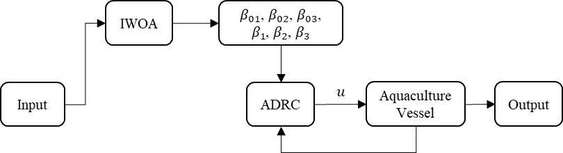
The function of the Improved Whale Optimization Algorithm (IWOA) is to optimize and tune the gain parameters in the Extended State Observer (ESO) of the Active Disturbance Rejection Controller (ADRC). The goal is to find a parameter combination that minimizes the absolute value of the system error, specifically using the minimum value of the Integral of Absolute Error (IAE) function (as shown in Equation 25) as the objective function for optimization.

$$\begin{array}{r} ITE = \frac{1}{n}\sum_{i = 1}^{n}\left( y_{i} - {\widehat{y}}_{i} \right)^{2}\tag{25} \end{array}$$

In this case, $y_{i}$ represents the actual output, ${\widehat{y}}_{i}$ is the desired output, and $n$ is the required population size for the IWOA. The maximum number of iterations $t_{\max}$=500, is set as the termination condition for the IWOA optimization. The process for optimizing the ADRC parameters in this study is illustrated in Figure 11.

The relevant parameters of the aquaculture vessel are shown in Table 3.

Using the ship’s relevant parameters described in Table 3, combined with the multiple regression analysis formula obtained by Zhou Zhaoming for the Moriya diagram in Japan²⁴ and the relevant hydrodynamic derivative formulas,^25–27 an estimate is made. Additionally, to verify the simulation experiment, the corresponding physical quantities are non-dimensionalized according to the “Prime System of SNAME²⁸”. Finally, the non-dimensional mass moment of inertia matrix and damping coefficient matrix of the vessel are calculated as shown in Equation (26):

$$\begin{array}{r} \left\{ \begin{array}{r} M = \begin{bmatrix} 6.2754 & 0 & 0 \\ 0 & 1.3723 & - 0.2437 \\ 0 & - 0.2437 & 0.2577 \end{bmatrix} \\ D = \begin{bmatrix} 1.2791 & 0 & 0 \\ 0 & 2.6297 & - 0.2533 \\ 0 & - 0.2224 & - 0.1305 \end{bmatrix} \end{array} \right.\ \tag{26} \end{array}$$

Assuming the ship starts from the current position $\eta_{0} = (0,0,0)^{T}$, to the desired position $\eta_{e} = (50,30,11.5)^{T}$. To verify the effectiveness of the proposed control algorithm, simulations are conducted in two modes: without disturbances and with disturbances. These are compared with traditional algorithms and other active disturbance rejection control (ADRC) algorithms used in the literature. Since the improved GWO adopted in Reference 1²⁹ is used for optimizing the ADRC in the DP system, it is taken as a reference for comparison in this simulation. The simulation results of the aquaculture support vessel DP system ADRC optimized by IWOA, traditional GA, WOA, and GWO are shown in Figures 12 to 14, with the data comparison presented in Table 4.

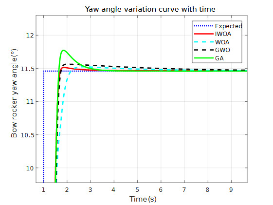
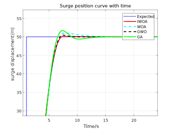
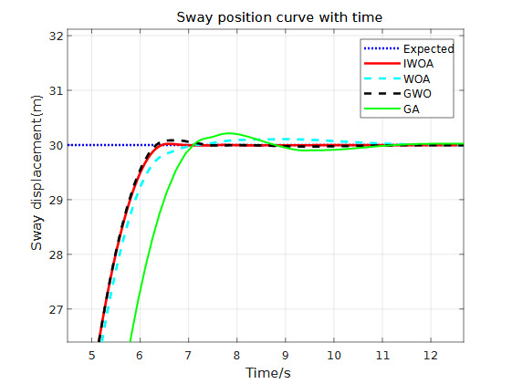
From the simulation results and Table 4 above, the following can be observed: (1) Figures 12 to 14 show the simulation results of the ship’s yaw, surge, and sway motions in calm water without disturbances. It can be seen from the figures that the ADRC controllers optimized by all four algorithms are able to control the ship to reach the desired position effectively.

According to the simulation data comparison in Table 4, the IWOA-ADRC optimized system has the smallest overshoot. In the yaw angle response, the system’s overshoot is reduced by 76%, 35%, and 95% compared to the GWO-ADRC, WOA-ADRC, and GA-ADRC methods, respectively. From Figures 12 and 13, it can be observed that the GA-ADRC method does not reach stability in the surge and sway directions within a short period, exhibiting slow convergence and oscillations. This not only significantly delays the system’s stabilization time but also causes system vibrations. The WOA-ADRC method has slower response speeds in the yaw angle and sway directions compared to other methods. In the sway response, it takes too long (about 11s) to stabilize, similar to GA-ADRC, showing poor speed and stability. The method from Reference 1 (GWO-ADRC) has faster response and convergence rates in the surge and sway directions, demonstrating certain speed and stability advantages. However, in the yaw angle response, the system stabilization time is too long, which may lead to instability. In comparison, the IWOA-ADRC method reduces the system’s overshoot by over 60% in all three degrees of freedom compared to the method in Reference 1, improving system stability and steady-state accuracy. Moreover, it achieves the desired target and stabilizes in the shortest time among the four methods. Therefore, under disturbance-free conditions, the IWOA-ADRC system has the fastest response speed and the best stability.

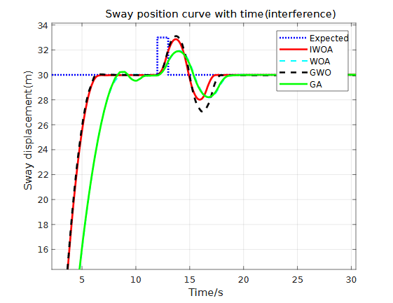
Considering that environmental disturbances are always present at sea, and internal liquid sloshing in the aquaculture support vessel can also generate disturbance signals, a step function is introduced at 12 seconds in the simulation to simulate the disturbances encountered during ship navigation. The final comparison results are shown in Figures 15 to 17, and the simulation data with disturbances are presented in Table 5.

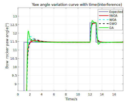
Figures 15 to 17 show the simulation results of the system under the influence of disturbances. From the figures, it can be observed that the control systems optimized by all four algorithms are able to restore stability after a certain period of disturbance, demonstrating a certain level of disturbance rejection capability. The experimental data comparison is presented in Table 5. It can be found that in the yaw angle response, the IWOA-ADRC method reduces the system’s overshoot by 74%, 86%, and 93% compared to the GWO-ADRC, WOA-ADRC, and GA-ADRC methods, respectively.

In the surge direction response curve, the GA-ADRC and WOA-ADRC methods both achieve stability before the disturbance. The overshoot values of the IWOA-ADRC and GWO-ADRC methods are similar. After the disturbance, the IWOA-ADRC method restores the system’s longitudinal stability at the fastest speed (4.721s after the disturbance), demonstrating its rapid response capability.

In the sway direction response curve, after the disturbance is introduced, both the GA-ADRC and WOA-ADRC methods respond more slowly (approximately 2 seconds later than the previous two methods) and exhibit some steady-state error. The IWOA-ADRC and GWO-ADRC methods have the fastest initial response and shorter times to restore lateral stability (4.311s and 4.975s after disturbance, respectively). However, the GWO-ADRC method has a larger overshoot. In contrast, the IWOA-ADRC method reduces the system’s overshoot by up to 10%.

It can be concluded that the IWOA-ADRC method can respond quickly after system disturbances and maintain good steady-state accuracy, enhancing both the system’s speed and control precision.

Discussion

To address the uncertainties in the vessel model and the difficulties in modeling caused by external environmental disturbances and internal fluid disturbances in deep-sea aquaculture working ships’ dynamic positioning (DP), a DP controller based on Improved Active Disturbance Rejection Control (IADRC) has been designed. Additionally, the Improved Whale Optimization Algorithm (IWOA) has been incorporated to overcome the challenges of parameter tuning for the DP controller.

According to the Simulink simulation results from the previous chapter, the IWOA-IADRC control strategy reduces the system overshoot ratio by over 70% in both disturbance-free and disturbed scenarios compared to the GWO-IADRC strategy used in Reference 1. Specifically, the overshoot reduction rates for the longitudinal and lateral response curves under disturbance-free conditions are approximately 80% and 75%, respectively. After disturbance, the IWOA-IADRC strategy stabilizes the longitudinal and lateral responses 0.423 seconds and 0.664 seconds faster than the GWO-IADRC strategy. Ultimately, the designed DP controller demonstrates superior response speed, stronger disturbance rejection capability, and enhanced dynamic performance compared to the WOA-IADRC, GWO-IADRC, and GA-IADRC-based DP controllers, ensuring the vessel’s stability and resilience against disturbances.

The main breakthroughs and shortcomings of this study are as follows:

1. Improved the ADRC system structure by adding a first-order integral gain system compared to traditional nonlinear state control. This effectively enhanced the system’s stability and tracking accuracy but reduced its response speed. Further improvements are needed for scenarios with high demands on system response speed, such as: Improved the performance of the Extended State Observer (ESO), enhancing the observation and compensation of disturbances.

2. In parameter tuning, an IWOA optimization algorithm was designed, which effectively addressed the issues of insufficient convergence speed and optimization accuracy in the traditional WOA algorithm when applied to the IADRC controller. This improvement increased the efficiency of system parameter optimization and control effects. However, the introduced chaotic search strategy, while enhancing the probability of avoiding local optima, may lead to long processing times and a sharp decline in optimization effectiveness in scenarios with large spaces and numerous variables. To effectively address this issue in subsequent studies, a co-evolutionary strategy can be introduced, where the population is divided into multiple subpopulations that evolve collaboratively.

3. Additionally, this study was unable to completely eliminate phase lag in the processing of high-frequency noise interference. In the future, adaptive filtering or the incorporation of a phase compensation component in the filter design could be introduced to mitigate the lag effect.

---

Acknowledgments

This work was supported by Ministry of Agriculture and Rural Affairs Financial Projects. The funded projects are D220150.

Authors’ Contribution

Conceptualization: Chao Lyu (Lead). Data curation: Chao Lyu (Equal), Shuang Liu (Equal). Project administration: Chao Lyu (Lead). Formal Analysis: Chao Lyu (Equal), Si-Dong Zhao (Equal), Si-Dong Zhao (Lead). Investigation: Chao Lyu (Equal), Si-Dong Zhao (Equal). Writing – review & editing: Chao Lyu (Lead). Supervision: Chao Lyu (Equal), Shuang Liu (Equal). Software: Si-Dong Zhao (Lead). Methodology: Si-Dong Zhao (Lead). Validation: Si-Dong Zhao (Lead). Visualization: Si-Dong Zhao (Lead). Funding acquisition: Shuang Liu (Lead). Resources: Shuang Liu (Lead).

Competing of Interest – COPE

No competing interests were disclosed.

Ethical Conduct Approval – IACUC

This study did not involve human or animal subjects, and thus, no ethical approval was required. The study protocol adhered to the guidelines established by the journal.

Informed Consent Statement

All authors and institutions have confirmed this manuscript for publication.

Data Availability Statement

All are available upon reasonable request.