Study on the Approval Criteria for Fishing Vessel Main Engine Power Control Based on Main Engine Power Calculation Methods

undefined

Introduction

Ocean fishing is a significant component of China’s fishery economy. As of the end of 2020, the total num-ber of active fishing vessels in China was approximately 563,300, remaining at a high level, and the competition among ocean fishing industries is intense.¹ Meanwhile, the decline in marine fishery resources has exacerbated this situation, and the cost of fishing continues to rise.² To enhance their competitiveness, fishermen often illegally increase the main engine power of their vessels, which can lead to inadequate safety equipment as re-quired by the “Fisheries Vessel Inspection Regulations.” In the event of an emergency during navigation, this can easily result in accidents such as capsizing and loss of life.³ To protect fishery resources, control ocean fishing intensity, and promote sustainable utilization of fishery resources, China has implemented a fishing permit sys-tem since the 1980s, setting “entry requirements” for fishing. With the development of the times, regulations on the construction or renovation of motorized fishing vessels have been introduced. These regulations mandate strict control over the main engine power parameters of newly built or renovated vessels, requiring that such activities can only proceed after the dismantling of existing vessels has freed up power parameter indicators. For instance, if the available power parameter indicator is 100KW, the main engine power of the newly built or reno-vated vessel must not exceed 100KW. Without available power parameter indicators, new vessels or renovations cannot proceed. In this context, fishery managers need to review whether the proposed vessel meets the required power parameter indicators based on the plans and specifications provided by the fishermen. On the other hand, fishermen hope to meet the control requirements for main engine power while also improving vessel performance to enhance their fishing capacity, such as increasing speed. This has led to industry issues like “over-powered but under-reported” vessels and challenges for approval authorities in managing main engine power approvals.

Based on ship test data, researchers have proposed numerous methods for estimating ship power. However, due to differences in design materials, propeller structures, and ship shapes between these test ships and the ships to be designed, many researchers have tested these methods for their predictive accuracy across various types of ships. Liu, F.⁴ and others estimated the main engine power using the parent ship series fitting method and the Ohkubo Miho method under conditions of known displacement, maximum speed, and total length, verifying the effectiveness of the estimation results through comparative analysis. Zhang Baoji⁵ compared various methods for estimating power in oil tankers, plotting graphs of effective power against speed, and found the Ayre method to be more effective when compared to experimental values. Deng Lili⁶ and others explored the adaptability of different methods for power estimation in fishery administration vessels. Ding, S.⁷ and others conducted power estimation through resistance and propulsion prediction, although the model was precise, the calculations were complex. Tu Haiwen⁸ evaluated the estimation accuracy of the original Admiralty coefficient formula based on data from container ships. An improved formula was proposed, which was proven to be more accurate than the original formula.

Meanwhile, as ships are gradually equipped with onboard data collection systems, shipowners, operators, and naval architects can utilize this data to improve vessels’ performance at sea. Zhang C⁹ and Moreira et al.¹⁰ applied machine learning to predict ship power using in-service data, but the effectiveness of these power prediction models largely depends on the quantity and quality of training data, and machine learning models per-form poorly in extrapolation. Furthermore, machine learning models are often viewed as “black boxes,” with us-ers knowing little about the reasons behind predictions. In this case, providing a degree of interpretability to the model can enhance user trust.¹¹ For example, CFD simulations validated by model test results have traditional-ly been used to predict ship power.¹² However, these methods require substantial time and resources, detailed ship and propeller geometry information, and experienced users to obtain reliable results.

Since the estimation of ship main engine power is crucial for calculating the effective power and propulsion efficiency of fishing vessels,¹³ and given that hull form data is not available during fishing vessel registration, the effective power of fishing vessels cannot be determined through ship model tests or simulation calculations to determine resistance, but can only be roughly estimated.¹⁴ Researching fishing vessel power estimation methods and their accuracy can provide reference for detecting whether the actual main engine power required by fishing vessels is consistent with the control index requirements for main engine power.

Numerous researchers and scholars have contributed to the field of power estimation, yet there remains a lack of a comprehensive summary and analysis of main engine power estimation methods specific to fishing vessels. This study aims to address this gap by presenting a summary, comparison, and analysis of fishing vessel main engine power estimation methods through example calculations. The goal is to facilitate a solution for the compatibility issue between approved power and actual power levels aboard fishing vessels.

Materials and Methods

Methods for estimating the effective power of fishing vessels

Fishing vessel effective power estimation is a crucial aspect of main engine power estimation. The effective power required by a fishing vessel encompasses the power needed to overcome resistance while sailing, which can enhance the vessel’s resistance performance. Presently, methods employed for calculating the effective pow-er of fishing vessels include the Navy coefficient method, the Japanese effective horsepower estimation atlas method, The Pavmiri method, the stern slipway trawler ship model series test, The Durst method, TAYLOR’s esti-mation method, Aiyah method, others. To accurately estimate main engine power, it is essential to analyze the characteristics and applications of these effective power estimation methods.

Department of the Navy coefficient method

The Department of the Navy coefficient, a pioneering drag approximation algorithm, relies primarily on the similarity of the inspected ship to the parent ship in terms of ship type, main scale data, Reynolds number, and Froude number for computational accuracy. The Department of the Navy factor is defined as:

$$C = \frac{\Delta^{\frac{2}{3}}V}{P_{E}} \tag{1}$$

Where: ∆ is the displacement in t; V is the speed in kn; and PE is the effective power in kW (HP).

When replaced P_E by the host power P, the Admiralty factor can be expressed as:

$$C = \frac{\Delta^{\frac{2}{3}}V}{P} \tag{2}$$

The constants C_E and C in Eq. (1) and Eq. (2) have slightly different meanings, with the former reflecting the drag performance of the ship and the latter reflecting the combined performance of drag and propulsion.

The main engine power of the inspected ship can be estimated using the coefficient provided by the Department of the Navy. The key factor is the type of mother ship, which should have a similar number of Fu Ruide as the inspected ship, along with similar scale and speed. By applying formula (1) to the mother ship’s data, the Department of the Navy coefficient for the inspected vessel can be determined, thereby obtaining the main engine power of the inspected ship.

$$P = C \cdot \Delta^{\frac{2}{3}}V \tag{3}$$

To employ this formula, certain data is necessary, including the displacement (Δ), the design speed (V), and the naval coefficient (C) of the fishing vessel.

Japan Effective Horsepower Estimation Method

Jun Takagi^15,16 and colleagues developed a set of charts for calculating the effective horsepower of fishing vessels by conducting a series of ship model tests, using a standard 95-ton wooden skipjack tuna fishing vessel as the mother model. Kazuo Ito¹⁷ adapted these charts in 1963 to simplify the calculation process.

The estimation formula is:

$$EHP = \left( E_{0} + \bigtriangleup E \right)\Delta\sqrt{L} \tag{4}$$

Where: EHP for the effective power, unit horsepower (metric); for the displacement ∆, unit t; for the length of the ship L, unit m; for the horsepower coefficient $E_{0}$ (L=30 ), according to, $V/\sqrt{Lg}$,$\ \overline{V}/{(L/10)}^{3}$, C_p, B/T, and other values according to the chart to find; for the horsepower correction coefficient$\bigtriangleup E$, which is calculated by the formula:

$$\bigtriangleup E = K_{L} \times K_{\text{v}}/\sqrt{\Delta} \tag{5}$$

Where K_L is the length correction factor, can check the literature.¹⁴ Generally L = 30m, K_L = 0 In the actual design of L = 20 - 50m range, the error is very small, and can not be corrected; K_V for the speed correction coefficient, from Table 1.

Scope of application for this atlas:

$$L = 10\sim 60m;$$

$$C_{p} = 0.55\sim 0.75;$$

$$\frac{V}{\sqrt{\left( \frac{L}{10} \right)^{3}}} = 6.0\sim 14.0;$$

$$\frac{B}{T} = 2.2\sim 3.0;$$

$$F_{r} = \frac{V}{\sqrt{gL}} = 0.20\sim 0.38;$$

To employ this formula, certain data is necessary, including the length of the column (L), the velocity (V), the width of the ship (B), the design draft (T), displacement (Δ), and the squared coefficient (C_p) of the fishing vessel.

The Pavmiri method

After analyzing and organizing information from a large number of ship models and real ships, Pavmir developed the method for determining the effective horsepower,¹⁸ which is expressed as follows:

$$P_{E} = \Delta/L_{WL} \cdot V^{3}/(C\lambda\left( 1 + K_{a} \right)\sqrt{\psi}) \tag{6}$$

where P_E is the effective horsepower (effective power is P_E/1.36) including the attachment, in horsepower (metric); ∆ is the displacement, in t; L_WL is the waterline length, in m; V is the speed, in kn; and Ka is a coefficient that takes into account the effect of the attachment on the drag, which is found in Table 2.

$\psi$ is the fertility coefficient of the hull, 𝜓 = 10𝐵/𝐿_𝑊𝐿𝐶_𝑏; 𝜆 is the correction factor for length, $\lambda\ = \ 0.7\ + \ 0.3\sqrt{L_{WL}/100}$, and the length is not corrected if the waterline is longer than 100 m. C is the correction factor for the length by the equivalent rate$V^{\prime}$ ($V^{\prime} = \ V\sqrt{\psi/L_{WL}}$) and a coefficient determined by the fertilization factor 𝜓, which can be found in the literature¹⁵ in Fig.

The scope of application of the method is:

$$\begin{array}{r} \psi = 0.35\sim 1.20; \\ B/T = 1.5\sim 3.5; \\ B/L = 0.09\sim 0.25; \\ C_{b} = 0.35\sim 0.80. \end{array}$$

To utilize this formula, a set of data is required, including the waterline length (L_WL), velocity (V), ship width (B), design draft (T), displacement (Δ), and squareness coefficient (C_b) of the fishing vessel.

Stern Slipway Trawler Vessel Model Series Tests

The UK published the results of a series of stern-slip trawler ship modeling trials with drag calculation data in 1974. The main objective of these trials was to provide useful drag information for design professionals working on the development of stern slipway trawlers.¹⁹ The dissemination of this test data is intended to serve as a reference for further improvement and optimization of the design of stern slipway fishing trawlers.

The test vessel values are shown in Table 3.

Three ship models, 1114, 1115, and 1116, were generated using the moving cross-section method to obtain the cross-section area curves of a series of changing ship models based on changes in the mother ship. The parameters for these ship models are presented in Table 4.

Based on the test results, both the stern-slip and outboard trawlers show a similar trend in the longitudinal position of the optical drag center of buoyancy. The longitudinal position of the optimal center of buoyancy can be determined using the following equation:

$$X_{b} = \frac{1 - V_{200}}{3} \tag{7}$$

Where: The longitudinal position of the center of buoyancy is expressed in percent of inter-length between perpendiculars, with negative values indicating a position behind amidships. V₂₀₀ represents the speed in knots of a stern-slip trawler with an inter-length between perpendiculars of 200 feet.

The drag coefficients are adopted from Rudolf Fu’s factor less drag coefficients © I. e:

$$ⓒ = \frac{427.1P_{EHP}}{\Delta^{\frac{2}{3}}V^{3}} \tag{8}$$

where: EHP denotes effective horsepower, measured in imperial horsepower; displacement is expressed in tons (with 1 metric ton equaling 1.016 tons); and the speed is measured in knots.

The effective horsepower estimation formula is expressed as follows:

$$P_{E H P}=\frac{\Delta^{2 / 3} V^3 \subset}{427.1} \tag{9}$$

where: EHP is the effective horsepower, the unit imperial horsepower, is the displacement, the unit ton (1 metric ton = 1.016 tons), is the speed, the unit knot.

Considering the change in drag coefficient © caused by the change of ship width and draft, the Mumford Indices are used to derive,²⁰ I. e：

$$P_{EHP} \propto B^{x}T^{y} \tag{10}$$

x and y in the above equation vary with $V/\sqrt{L}$.

According to Eq. (10) and the principle that B and T change assuming that the length of the ship does not change, Eq. (9) can be written as follows, namely:

$$ⓒ \propto B^{x}T^{y} \tag{11}$$

© is the drag coefficient in equations (7) and (8); B is the width of the ship, in feet; T is the design draft, in feet; x and y are the door indices and vary with $V/\sqrt{L}$.

In the effective horsepower estimation, the © value of the ship to be calculated is obtained as follows, I. e:

$$\begin{align} ⓒ &= ⓒ_{b} \times X_{bC} \times \text{C}_{bC} \\&\quad\times \left( \frac{B}{40} \right)^{x - 2/3} \times \left( \frac{T}{16.5} \right)^{y - 2/3} \end{align} \tag{12}$$

where: $ⓒ_{b}$is the drag coefficient of the ship’s inter-length between perpendiculars of 200 feet, which can be obtained according to the interpolation value in Table 5, if the inter-length between perpendiculars is not equal to 200 feet, it needs to be included in the correction value S_SFC calculated according to Eq. (13); The X_bc is obtained according to the literature of Jia, F²⁰; C_bc is obtained according to the literature of Jia, F²⁰; B is the beam of the calculated ship, in feet; T is the draft of the calculated ship, in feet; x and y are the door indices and are found in Table 6.

When the length between the columns of the calculated ship is not equal to 200 feet, a surface friction correction is required, the correction value of which is:

$$S_{SFC} = \left( O_{CC} - O_{200} \right)ⓢⓘ^{- 0.175} \tag{13}$$

Where: S_SFC is the surface friction correction value: O is found from Table 7 according to the length between columns; $ⓢ$ can be obtained from Eq. (14); $ⓘ$ is obtained by Eq. (15);

$$\begin{align}ⓢ &= \frac{S}{\nabla^{\frac{2}{3}}} = 5.0699 - 0.5657C_{b} \\&\quad+ 0.0217\left( \frac{L_{PP}}{B} \right) + 0.0752\left( \frac{B}{T} \right) \end{align}\tag{14}$$

where: C_b is the square coefficient; L_BP inter-length between perpendiculars, in feet; B is the width of the ship, in feet; T is the design draft in feet.

$$ⓘ = 1.055\frac{V}{\sqrt{L_{PP}}} \tag{15}$$

where: V is the speed, and the unit section; L_BP is the length between the columns, and the unit is feet.

When the length of the ship’s columns differs from 200 feet, the value of ©_b can be derived from Table 6. The value of its modified version (SFC) is calculated using Eq. (13), and then substituted into Eq. (12) to obtain the computed ship’s drag coefficient ©. This enables the calculation of the effective horsepower according to Eq. (9). The scope of application is as follows:

$$\begin{array}{r} V = 9\sim 17Kn; \\ X_{b} = 1.5\sim 6\% L_{PP}; \\ C_{b} = 0.49\sim 0.60. \end{array}$$

To employ this formula, certain data is necessary, including the length of the column (L), the width of the ship (B), the design draft (T), the velocity (V), the displacement (D), and the squared coefficient (C_b) of the fishing vessel. The power derived from this formula is in imperial horsepower, which must be converted.

Durst method

Doust (Doust)²⁰ and others statistically analyzed the British National Institute of Physics Ship Department of the first test pool, the resistance test results of about 130 fishing boats, selected the aspect ratio L_PP/B; width draft ratio L/B; clock profile coefficient C_M; prismatic coefficient C_p; longitudinal position of the center of gravity X_b; full waterline half-advancement 1/2 a_e and so on, six kinds of parameter constitutes the resistance function of the fishing boat, and put the fishing boat resistance with the use of these six kinds of parameters to produce a set of charts, divided into four groups of parameters. The resistance of the fishing vessel is divided into four groups of parameters by using these six parameters to produce a set of plots, the first group of plots of F₁ by $V/\sqrt{L_{PP}}$, B/T, Cp decision; the second group of plots of F₂ by $V/\sqrt{L_{PP}}$, LCB, C_p decision; the third group of plots of F₃ by $V/\sqrt{L_{PP}}$, C_p, 1/2 a_e decision; the fourth group of plots of F₄ by $V/\sqrt{L_{PP}}$, C_M decision.

When calculating the effective power of the tested fishing vessel, according to the main parameters of the tested vessel, the value of the drag coefficient $C_{f(200)} = RL/(\mathrm{\Delta} \cdot V^{2})$ is calculated according to the chart with the length of the vessel equal to the length of 200 feet between the columns, and then the friction drag coefficient is corrected according to the actual length of the vessel, so that the C_R of the “calculated vessel” is:

$$C_{f} = C_{f(200)} + \delta_{1} \tag{16}$$

$$\delta_{1} = \frac{152.2 \times S_{SFC}}{\Delta_{(200)}^{\frac{1}{3}}} \tag{17}$$

Where: $C_{R(200)}$ is the drag coefficient for a ship with a length between perpendiculars of 200 feet; $\delta_{1}$ is the correction for C_R due to the calculation of a ship with a length between perpendiculars not equal to 200 feet, which can be obtained from equation (17); and S_SFC is the correction for surface friction of the ship under test with a length between perpendiculars not equal to 200 feet, which can be calculated from equation (13).

The drag coefficient C_R for the length of the ship under survey is equivalent to 200 feet between the columns, and the formula is as follows:

$$C_{f(200)} = F_{1} + F_{2} + F_{3} + F_{4} \tag{18}$$

The values of F₁、F₂、F₃、F₄ were found separately from the four sets of plots.

And then the effective horsepower of the ship to be surveyed is:

$$P_{EHP} = \frac{C_{R} \times \Delta \times V^{3}}{325.7 \times L_{PP}} \tag{19}$$

Where: EHP is the effective horsepower in horsepower (imperial); C_R is the drag coefficient of the vessel under test; Δ is the displacement of the vessel under test in British tons; and L_BP is the length between the columns of the vessel under test in feet.

The graph and regression equation obtained by Doust from the statistical analysis of fishing vessel resistance data are limited in use, and their application ranges are as follows:

$$\begin{array}{r} C_{P} = 0.60\sim 0.705; \\ B/T = 2.0\sim 2.6; \\ X_{b} = 0\sim 6\% L_{PP}(\text{aft amidships})； \\ 1/2a_{e} = 5.0\sim 30.0; \\ C_{M} = 0.81\sim 0.91。 \end{array}$$

To employ this formula, certain data is necessary, including the fishing vessel’s inter-length between perpendiculars (L_PP), width (B), design draft (T), speed (V), displacement (Δ), clock profile coefficient (C_M), prismatic coefficient (C_p), full-load discharge line half-entry angle (1/2 a_e), and other data, and this formula to find the power for the imperial horsepower needs to be converted to it.

TAYLOR’s estimation method

TAYLOR’s estimation method is based on TAYLOR’s standard series of ship model test results, TAYLOR’s estimation method will be divided into residual resistance and friction resistance are estimated separately. 1954 Gattler through the analysis of TAYLOR’s standard group of resistance data, in the former based on the water temperature, laminar currents, and restrictions on the channel of the influence of the respective correction, organized a set of dimensionless residual resistance coefficient charts, expanding the scope of use of the method of TAYLOR’s estimate. The estimation method is also called Tylor-Gettler method.²¹ The calculation process is as follows:

1)Specify the ship type parameter values of the tested ship: B/T, C_p, $\nabla/L^{3}$, and F_r.

2)Get the wet area coefficient C_S

The wet area coefficient can be obtained indirectly from the ship shape diagram. If no profile is available, it can be approximated that the wet area of the ship under test is equal to that of the standard ship type. According to the given B/T value, select the two C_S graphs closest to it and find the C_S value. Then, the C_S value of the standard ship type is calculated by linear interpolation for the given parameter values.

3)Calculate the friction resistance coefficient C_f value

The value of the friction resistance coefficient C_f can be obtained by Sonhai’s plate formula, or by looking up the Reynolds number table or directly calculating.

$$C_{f} = 0.4631/{(\lg Re)}^{2.6} \tag{20}$$

$$Re = \frac{vL_{WL}}{\upsilon} \tag{21}$$

The variables are defined as follows: Re represents Reynolds number; v represents the flow rate of the fluid; L_WL represents the waterline length; $\upsilon$ represents the kinematic viscosity coefficient. When the seawater represents 15 degrees Celsius, $\upsilon = {1.1883}^{- 6}$.

4)Find the residual drag coefficient

According to the parameters B/T, C_p, $\nabla/L^{3}$and F_r values of the measured ship, the corresponding C_r graph is selected and the C_r value is obtained by interpolation. If the wet area $S^{\prime}$ of the ship under test is known, then the wet area coefficient ${C_{s}}^{\prime}$ of the real ship can be obtained as:

$$C_{\text{s}}^{\prime} = \frac{S^{\prime}}{\sqrt{\nabla L}} \tag{22}$$

Where: S’ is the wet area of the ship under test, unit m²; ∇ The volume of the vessel under test, in m³; L for Captain, unit m.

When C_s is different from the wet area coefficient C_s of the standard ship type, the residual resistance coefficient value C_r needs to be corrected, and the corrected residual resistance coefficient ${C_{r}}^{\prime}$of the real ship is:

$$C_{r}^{\prime} = C_{r}\frac{C_{s}}{C_{s}^{\prime}} \tag{23}$$

When the wet area coefficient of the ship is unknown, it can be assumed that ${C_{s}}^{\prime} = C_{s}$, then:

$$C_{r}^{\prime} = C_{r} \tag{24}$$

5) Find the value of total resistance and effective power.

The total resistance coefficient C_ts is:

$$C_{ts} = C_{r}^{\prime} + C_{f} + \bigtriangleup C_{f} \tag{25}$$

Where: C_f is the friction resistance coefficient; C_f is calculated according to equation (20). $\bigtriangleup C_{f}$is the added value of roughness, generally $0.4 \times 10^{3}$.

Total resistance is:

$$R_{ts} = C_{ts}\frac{1}{2}\rho V^{2}S' \tag{26}$$

The effective power is:

$$P_{E} = \frac{R_{ts}V}{1000} \tag{27}$$

The application scope of this method is shown in Table 8.

To employ this formula, certain data is necessary, including the fishing vessel’s length (L), ship width (B), the design draft (T), the speed (V), displacement (Δ), square coefficient (C_b), prismatic coefficient (Cp), and other data.

Aiyah method

Aiya analyzed the results of a large number of ship models and real ship tests, drew the curve chart for resistance estimation, and then directly estimated the effective power for the standard ship model; then corrected one by one according to the differences between the tested ship and the standard ship model, and finally obtained the effective power value of the tested ship.

The corresponding parameters of Aiyah law standard ship type are:

(1) The formula for finding the standard square coefficient $C_{bc}$is as follows:

Single oar vessel:$C_{bc} = 1.08 - 1.68F_{r}$;

double-oared vessel: $C_{bc} = 1.09 - 1.68F_{r}$.

(2) Standard width-draft ratio: B/T=2.0.

(3) Longitudinal position of standard center of buoyancy

(4) Standard waterline length: $L_{WL} = 1.025L_{PP}$

The effective power P_E (kW) formula of the standard ship type of Aija method is:

$$P_{E} = \frac{\Delta^{0.64}V_{S}^{3}}{C_{0}} \times 0.735 \tag{28}$$

Where: V_s for the hydrostatic test speed, the unit of knots; Δ for the displacement, the unit of t, the displacement of the index of Δ due to the frictional resistance with the scale of the growth than the residual resistance with the scale of the growth of the slower and take 0.64; C₀ for the length of the displacement coefficient can be based on the length of the$\ L\ /\mathrm{\Delta}^{1/3}$ and the speed of the ratio of length of the $V\ /\sqrt{L}$ (or F_r) can be looked up in Articles by Sheng, Z.B. to get.²¹

Power estimation for non-standard ship types requires corrections to the values in Eq. (28). Corrections are made in four areas: squareness factor, width-to-draft ratio, longitudinal position of the center of gravity, and waterline length.

1)Correction of square coefficient

When the square coefficient $C_{b}$ of the measured fishing vessel is different from the standard square coefficient $C_{bc}$, C₀ is corrected by adding a correction quantity $\bigtriangleup_{1}$.

When C_b>C_bc

$$\bigtriangleup_{1} = - 3 \times C_{b}\frac{C_{b} - C_{bc}}{C_{bc}}C_{0} \tag{29}$$

When C_b≤C_bc

$$\bigtriangleup_{1} = C_{0} \times K_{bc} \tag{30}$$

2)Width draft ratio correction

When the width draft ratio of the measured fishing vessel is not 2.0, the correction of C₀ is realized by adding another correction. $\bigtriangleup_{2}$

This $\bigtriangleup_{2}$ is:

$$\bigtriangleup_{2} = - 10 \times C_{b}(B/T - 2)\% \times (C_{0} + \bigtriangleup_{1}) \tag{31}$$

3)Longitudinal position correction of center of buoyancy

If the longitudinal position of the center of buoyancy of the ship under test is not in the standard position, another correction quantity $\bigtriangleup_{3}$needs to be added for correction. To confirm the value of $\bigtriangleup_{3}$, $\left( \bigtriangleup_{3} \right)_{0}$ should be computed according to Eq. (32).

$$\left( \bigtriangleup_{3} \right)_{0} = \left( C_{0} + \bigtriangleup_{1} + \bigtriangleup_{2} \right) \times K_{\text{xc}} \tag{32}$$

Where: $K_{xc}$ is the percentage reduction, which can be obtained from the literature²¹：

When $\bigtriangleup_{1}$<0,then$\bigtriangleup_{3} = - \left( \bigtriangleup_{3} \right)_{0}$;

When $\bigtriangleup_{1}$<0,and $\left| \left( \bigtriangleup_{3} \right)_{0} \right| \leq \bigtriangleup_{1}$,then $\bigtriangleup_{3} = 0$;

When $\bigtriangleup_{1}$<0,and $\left| \left( \bigtriangleup_{3} \right)_{0} \right| > \bigtriangleup_{1}$,then $\bigtriangleup_{3} = - \left| \left( \bigtriangleup_{3} \right)_{0} \right| - \bigtriangleup_{1}$.

4)Correction of waterline length

If the waterline length of the measured vessel L_WL is not equal to the standard waterline length, further correction is required. The formula for the correction value D is:

$$\begin{align}\bigtriangleup_{4} &= \frac{L_{WL} - 1.025L_{BP}}{1.025L_{BP}} \\&\quad\times \left( C_{0} + \bigtriangleup_{1} + \bigtriangleup_{2} + \bigtriangleup_{3} \right) \end{align}\tag{33}$$

The fully corrected coefficient $C_{1} = C_{0} + \bigtriangleup_{1} + \bigtriangleup_{2} + \bigtriangleup_{3} + \bigtriangleup_{4}$. The effective power of the ship under test is:

$$P_{E} = \Delta^{0.64}V_{S}^{3}/C_{1} \times 0.735 \tag{34}$$

To employ this formula, certain data is necessary, including the fishing vessel’s waterline length (L), length between perpendiculars (L_PP), ship width (B), the design draft (T), speed (V), displacement (Δ), square coefficient (C_b), prismatic coefficient (C_p), and other data.

Summary

The estimation of effective power can be categorized into two methods: one involves using empirical formulas or parameters from the main ship to directly estimate total resistance or effective power, while the other method involves analyzing a large number of ship model test series and actual ship test voyage data to establish a series of charts for the ship model. This allows for the calculation of residual resistance and the use of corresponding plate formulas to calculate friction resistance, and ultimately the total effective power. The principle parameters of these methods are detailed in Table 9.

Estimation of main engine power using effective horsepower of fishing vessels

High-quality fishing vessels must prioritize navigation economy, low fuel consumption, and substantial towing power to withstand adverse sea conditions.²² This necessitates that the main engine of the fishing vessel can deliver the required power to ensure safe navigation. To standardize production, different legal navigation areas and operational requirements are delineated based on the fishing vessel’s power. Simultaneously, the number of crew members and safety equipment are stipulated according to the vessel’s power. Inaccurate main engine power poses a hidden danger to safe production, necessitating the improvement of accuracy in estimating the main engine power of fishing vessels. The propeller-driven host power of the fishing boat overcomes hull resistance, and by mapping the propeller series, the relationship between effective power and host power can be established to estimate the host power of the fishing boat.

Propeller design diagram

The propeller design atlas is a specialized compilation of geometric parameters related to performance, derived from open-water model tests of propellers. It provides the most suitable propeller performance index within the range of propeller information offered. This atlas is specifically applicable to the preliminary design of propellers for conventional ship types with relatively uniform companion currents. Currently, most ship propeller matching designs are based on series diagrams, such as B-8 series diagrams and MAU series diagrams, which have undergone extensive testing and refinement.²³ Additionally, some research organizations have incorporated computer technology into the calculation of propeller design atlases to achieve fast and accurate calculations. Fu Pinsen also presents specific methods of propeller selection through practical cases in his work.²⁴ Notably, the world’s leading propeller design atlases include the B-type propeller design atlas of the Netherlands and the AU-type propeller design atlas of Japan.

The interaction coefficient between propeller and hull is estimated

During operation, the propeller interact with the ship’s hull due to hydrodynamic effects, which can affect propeller efficiency and propulsion to some extent. In 1976, Kugr proposed a formula for estimating companion currents of single and double propeller cargo ships. In 1988, Schneekluth proposed a formula for estimating companion currents of single-propeller bulbous-tailed cargo ships. Additionally, Heckscher, Caldwell, Telfer, Papmeh, and other researchers have also made significant contributions in this area. Yaru Y²⁵ To study the effect of towed objects on the resistance of fishing vessels under different conditions. In particular, the study investigated changes in the ship’s resistance, rather than the additional load from the towed object; Although the interaction with Kelvin waves and towed objects was also studied. The aim is to understand best practices and provide guidance on tow length. Schneekluth²⁶ and others processed a large amount of ship model pool experimental data to study the impact of ship parameters, resulting in the development of a companion current estimation formula through regression analysis. In 1965, Koshiji Shigenobu proposed a formula for estimating companion currents under different loading conditions of fishing vessels.

Thrust derating refers to the additional hull thrust caused by the propeller working behind the ship, with the thrust derating coefficient representing the ratio of thrust derating to thrust. Determining the factors affecting the thrust reduction factor is highly complex and is typically determined based on ship model tests. However, it can also be approximated by empirical formulas. Commonly used estimation formulas include the Heckscher formula, Shang He formula, Gotebao formula, and Holtlow formula.²⁷ The thrust derating coefficient is significantly influenced by waves, and an increase in propeller load will result in a change in the thrust derating coefficient under actual working conditions.²⁸ Currently, most of our fishing vessels are small to medium-sized, and Hankschel’s formula is highly accurate for estimating the fraction of companion currents as well as the fraction of thrust derating for such vessels.

Heckscher wake coefficient estimation formula is:

$$w = 0.77C_{P} - 0.28 \tag{35}$$

Where: w is the fraction of flow and C_p is the prismatic coefficient.

Hecksher thrust reduction coefficient estimation formula is as follows:

$$t = 0.77C_{P} - 0.30 \tag{36}$$

Where: $t$ is the prismatic coefficient.

Estimation of host power using effective power

The propeller acts as a connection between the hull and the primary engine, and its open-water efficiency is determined by the ratio of the thrust produced by the propeller while in motion in the water to the energy it uses. The energy used by the propeller comes from the main engine. When the ship travels at a consistent speed, the thrust generated by the propeller is approximately equal to the resistance of the ship in the water. In simpler terms, the power produced by the propeller, PTE, is roughly equal to the effective power of the fishing vessel P_E.

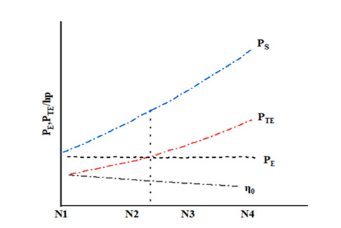
The atlas was determined based on the propeller type, blade number, and disk area ratio, and was calculated according to the steps outlined in Table 10. Assuming a range of propeller speeds, the results in Table 10 were obtained with speed N as the horizontal coordinate and P_S and P_TE as the longitudinal coordinates, respectively. The optimal speed is determined by the horizontal coordinate of the intersection point between the power P_TE supplied by the propeller and the effective power P_E of the fishing boat in Figure 1. The corresponding vertical coordinate on the P_S curve represents the estimated power of the main engine.

Where each parameter is defined as follows: $\eta_{H}$ represents is the hull efficiency; V is the ship speed, unit m/s; V_A represents the propeller feed speed, unit kn; B_P represents the force coefficient; N represents the propeller rotational speed, unit rpm; P_D represents the power received by the propeller in the open water, unit kW; P_S is the power of the main engine, unit kW; P_TE represents the calculated power that can be supplied by the propeller; $\eta_{s}$ represents the transmission efficiency of the shaft system; $\eta_{R}$ represents the relative rotational efficiency; $\eta_{0}$ represents the optimal efficiency of the propeller.

The fitting formula estimates the power of the main engine

Zhou Chunhui and colleagues²⁹ devised a model to predict a ship’s main engine power using data from the AIS database and the Yangtze River ship registration database. This method produced precise estimates owing to the robust relationship between main engine power and the ship’s dimensions. Nonetheless, the model necessitates a substantial volume of data and encompasses various undetermined parameters.

In this paper, we introduce the following relationship based on Fu Ruide’s resistance coefficient formula and the connection between main engine power and total ship resistance.

$$P_{S} \propto R_{t} \cdot V \tag{37}$$

$$R_{t} = ⓒ \cdot \pi/125 \cdot 1/2 \cdot \rho \cdot V^{2} \cdot \nabla^{\frac{2}{3}} \tag{38}$$

$$\nabla = C_{b} \cdot L \cdot B \cdot d \tag{39}$$

$$P_{S} \propto V^{3}(LBd)^{\frac{2}{3}} \tag{40}$$

Where the variables are defined as follows: © represents a constant, R_t represents the ship’s integrated resistance; ρ represents the density of seawater, unit kg/m³; V represents the speed, unit m/s; $\nabla$ represents the drainage volume, unit m³; $C_{b}$ represents the squareness coefficient; L represents the length of the ship, unit m; B represents the ship’s breadth, unit m; d represents the draft, unit m.

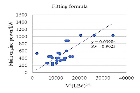
Based on the data of 33 fishing vessels (different types of fishing vessels) in the China Marine Fishing Vessel Atlas, a linear fitting curve was established with the main engine power P_S as the vertical coordinate and V³(LBd)^2/3 as the horizontal coordinate. As shown in Fig. 2:

Then the fitting formula $P_{S} = 0.0398 \cdot V^{3}(LBd)^{\frac{2}{3}}$can be obtained, in the process of fitting analysis, the decidable coefficient R² reacts to the percentage of the total variation that can be explained by the correlation in the fitting function, and the greater the percentage of the variation explained by the fitting curve, the more reliable the fit of the fitting function to the actual situation. From R²=0.9023 it can be seen that this linear equation has a reliable fit and this formula has some usability. At the same time, this formula contains more parameters of the main scale of the fishing vessel, and its results have a certain rationality.

When employing this method, the design speed Vs is substituted for the speed of the ship (V) the length between perpendiculars (L_BP) is utilized instead of the ship’s length (L), and the design draft (T) is used in place of the draft (d). The power obtained by this formula is in metric horsepower units, and thus requires conversion.

Host Power Audit Method

In 2020, Zhejiang Province issued a notice regarding the Management of the Fishing Vessel Fishing License. The notice stipulated restrictions on the use of the main engine power coefficient for applications related to the production, renewal, and reconstruction of main engine power for domestic marine fishing vessels. This re-striction requires that the ratio of the fishing vessel’s host engine power to the product of its length, width, and depth must fall within specific value ranges, detailed in Table 11.

The host power factor equation is:

$$Host\ power\ factor = \frac{P}{L \cdot B \cdot D} \tag{41}$$

The formula Eq. (41) is used to assess if the host power meets the audit requirements, but it does not accurately limit the main engine’s power. The parameters required for estimating the main engine power using this method include the host power factor, length (L), width (B), depth (D), and others. The coefficient can be calculated from the corresponding parameters provided by the fishing vessel to ensure compliance. By utilizing the vessel’s parameters, the coefficient range can be calculated to check if it meets the requirements. Simultaneously, it can also infer the coefficient for the main engine power of the fishing vessel. This formula, based on actual inspection values obtained from numerous audits, has led to the formulation of relevant regulations in Zhejiang Province. These regulations aim to enhance the approval process for fishing vessel main engine power, ensuring the alignment of approved power and actual power.

Results

This study utilizes an actual fishing vessel as a case study for estimation. Obtaining data such as mother ship displacement (Δ), design speed (V_S), naval coefficient (C), and others for different fishing vessels is challenging. Additionally, acquiring data for the longitudinal position of the center of gravity of the float is difficult, making the Tailor’s method less suitable as it is more appropriate for lean high-speed boats, whereas fishing vessels are predominantly low-speed boats. The research selects the Japanese fishing boat’s effective horsepower estimation method, the Pavmire method, the Aiyah method, and other approaches to assess the accuracy of estimating the main engine power of fishing boats. A comparative analysis with the fitting formula method and the main engine power audit method is also conducted. Data from fishing vessels in a province and the China Marine Fishing Vessel Atlas are included, as presented (Table 12).

The propeller power increases nonlinearly with rotational speed, and its efficiency sharply declines after reaching the peak value.³⁰ Therefore, when utilizing the effective horsepower estimation atlas of Japanese fishing vessels, Pavmire’s method, and Aiyah’s method, the appropriate range of rotational speed N in Table 10 should be considered, with the rotational speed N set at 100-300 r/min during the calculation process. The ship’s main engine power in (Table 12) is estimated using the fitting formula estimation equation of the law of the hour and the main engine power auditing method, with the results presented (Table 13).

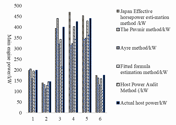
Comparing the above calculations with the actual results, the degree of difference is showned (Figure 3):

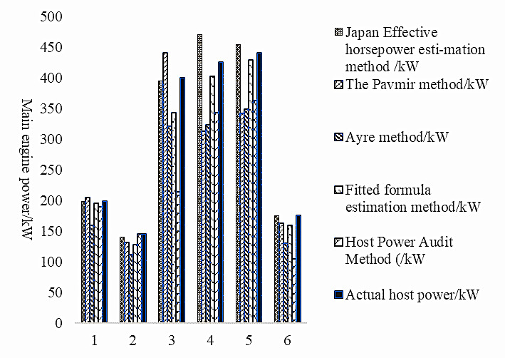
The comparative analysis in (Figure 3) reveals that the main engine estimated value obtained using the Japanese effective horsepower estimation method closely aligns with the actual power value. This suggests that the fishing vessel design enterprise may be using the Japanese mother ship model as a reference in their designs. In contrast, the values estimated using the Ayer method and the fitting formula method are both lower than the actual main engine power. Furthermore, considering the fishing vessel types, the estimated values of drift gillnet vessels exhibit closer proximity to the actual values compared to those of trawlers.

Upon reviewing (Figure 4), it is evident that the Pavmire method exhibits significant estimation error fluctuation, while the Aiya method yields errors ranging between 20% and 30%. The fitting formula method demonstrates a maximum error of approximately 15%. The host power auditing method shows minimal power estimation errors for some fishing vessels, although, for others, the estimated power versus actual power error is notably high, reaching up to 46%, thereby limiting the efficacy of the host power auditing for fishing vessels. In contrast, the Japanese Effective Horsepower Estimation Method closely aligns with the actual power, with a maximum error rate of around 10%.

To more comprehensively evaluate the performance of each method, we calculated the RMSE (Root Mean Square Error), MAE (Mean Absolute Error), MAPE (Mean Absolute Percentage Error), and MaxE (Maximum Error) for each method. The results are shown in the table below.

Japan Effective Horsepower method has a root mean square error (RMSE) of 19.13 kW, a mean absolute error (MAE) of 11.68 kW, a mean absolute percentage error (MAPE) of 3.21%, and a maximum error (MaxE) of 44.12 kW. This indicates excellent performance in error control, with significantly lower MAE and MAPE compared to other methods, showing high accuracy and consistency between predictions and actual values.

Pavmir Method has an RMSE of 63.92 kW, an MAE of 47.32 kW, a MAPE of 13.02%, and a maximum error of 112.88 kW. The larger error distribution, particularly in RMSE and MaxE, suggests that this method struggles with extreme values, resulting in lower precision and consistency.

Ayre Method has an RMSE of 71.20 kW, an MAE of 65.97 kW, a MAPE of 22.50%, and a maximum error of 102.89 kW. With a MAPE of 22.50%, this method shows relatively high relative error, making it less suitable for scenarios requiring high accuracy.

Fitted Formula Estimation has an RMSE of 29.94 kW, an MAE of 24.33 kW, a MAPE of 8.52%, and a maximum error of 60.62 kW. This method strikes a balance, with error metrics between Japan Effective Horsepower and other methods. Its MAPE of 8.52% indicates reliable relative error control, making it a viable secondary choice.

Host Power Audit has an RMSE of 93.67 kW, an MAE of 71.23 kW, a MAPE of 21.47%, and a maximum error of 185.63 kW. With the highest RMSE and MaxE among all methods, it shows significant deviation in predictions, especially with extreme values, indicating lower reliability.

In summary, the Japan Effective Horsepower method performs best across all error metrics, particularly with notably lower MAE and MAPE, making it ideal for scenarios requiring high precision. The Fitted Formula Estimation method is a good secondary option, with slightly higher errors but still maintaining good overall control. In contrast, the Pavmir Method, Ayre Method, and Host Power Audit have larger errors, especially in RMSE and maximum error, making them more suitable for applications with lower sensitivity to error.

Discussion

This paper provides a comprehensive overview of the existing methods for estimating the effective horsepower of fishing vessels and delves into the estimation of their main engine power. In addressing the challenge of power estimation for fishing vessels, the study considers the practical aspects of ship inspection and, in conjunction with existing calculation formulas, develops an estimation method for the main engine power of fishing vessels. The work conducted is as follows:

(1) Given the diverse array of fishing vessel types and the substantial variation in data among them, it is imperative to select an appropriate method for estimating main engine power to enhance the accuracy of estimation. This study comprehensively summarizes estimation methods suitable for determining the effective power of all types of fishing vessels.

(2) Notably, the study reveals that the Japanese fishing vessel’s effective horsepower estimation method, when combined with the propeller mapping method, yields greater reliability for estimating main engine power in small and medium-sized fishing vessels compared to other methods. Additionally, the fitting formula method demonstrates adaptability in estimating main engine power for different types of fishing vessels.

(3) Fishing vessel design and manufacturing enterprises generally do not specify the mother ship type used in the design of the fishing vessel. The mother ship type for the fishing vessel design can be inferred by comparing the calculation results and the corresponding formula. If the power of the fishing vessel in this study’s calculation closely resembles the results obtained by the Japanese effective horsepower estimation method, it suggests that the mother ship type of the fishing vessel design is referenced. Subsequently, the relationship between the main engine power and the main scale of the hull can be studied based on the characteristics of the mother ship type.

(4) Utilizing the findings of this study, the approval process for fishing vessel nets can achieve improved accuracy in auditing main engine power. This contributes to addressing the issue of discrepancies between the actual main scale of the fishing vessel and the approved power, providing valuable insights for mitigating the “big engine, small scale” dilemma.

In the future, the practicality of the Japanese effective horsepower estimation method will be further examined with more fishing vessel data. Additionally, a regression equation for estimating main engine power will be established based on the current fitting formula, combined with research on the characteristics of vessel engine-propeller matching and more fishing vessel data. This approach aims to achieve accurate and versatile estimation of main engine power for fishing vessels.

Despite its contributions, this study has several limitations. For example, the focus on small to medium-sized fishing vessels limits its applicability to other vessel types, and the reliance on data from specific regions (e.g., the China Marine Fishing Vessel Atlas) may not reflect global variations in vessel design and performance. Additionally, the lack of robust statistical validation or error analysis reduces the reliability of the proposed methods for broader application, and the limited sample size may not fully represent the diversity of fishing fleets. These limitations may affect the generalizability and precision of the findings. However, the findings remain valuable as they provide a foundation for improving fishing vessel power estimation methods and offer insights for addressing industry challenges.

---

Acknowledgments

This work was supported by The Fishery Administration Project of the Ministry of Agriculture and Rural Af-fairs: Offshore Fishing Vessel Performance Capacity Analysis Evaluation and Management. (D-8021-21-0076)

Authors’ Contribution – per CRediT

Conceptualization: Chao Lyu (Lead). Data curation: Chao Lyu (Equal), Shuang Liu (Equal). Formal Analysis: Chao Lyu (Lead). Project administration: Chao Lyu (Lead). Resources: Chao Lyu (Lead). Supervision: Chao Lyu (Lead). Writing – original draft: Chao Lyu (Equal), Yihe Shi (Equal). Writing – review & editing: Chao Lyu (Equal), Shuang Liu (Equal). Investigation: Yihe Shi (Lead). Methodology: Yihe Shi (Lead). Software: Yihe Shi (Lead). Validation: Yihe Shi (Lead). Visualization: Yihe Shi (Lead). Funding acquisition: Shuang Liu (Lead).

Competing of Interest – COPE

No competing interests were disclosed.

Ethical Conduct Approval – IACUC

There is no moral statement involved

Informed Consent Statement

All authors and institutions have confirmed this manuscript for publication.

Data Availability Statement

All are available upon reasonable request.