

Introduction
Stock enhancement, a pivotal strategy for fisheries restoration, has long been a subject of extensive debate. Extensive research has demonstrated that the widespread release of hatchery-reared fish into the natural environments can introduce significant genetic and ecological risks.1,2 These risks are primarily linked to declines in genetic diversity within hatchery populations.3 A marked reduction in genetic diversity can lead to severe consequences, such as diminished adaptive potential, increased homozygosity, altered phenotypes, and reduced overall fitness.4 To address these risks, hatcheries commonly source broodstock directly from wild populations rather than relying on successive generations of hatchery-born individuals. Nevertheless, ensuring high levels of genetic diversity among offspring remains an ongoing challenge. Two primary factors contribute to this issue: the limited availability of wild broodstock and a lower-than-expected number of effective breeders, both of which result in reduced genetic variation in offspring populations.
The selection of unrelated individuals for broodstock formation is widely recognized as a robust strategy for maintaining genetic diversity.5 Precise kinship estimation plays a critical role in facilitating informed decision-making during broodstock selection. Over the past few years, microsatellite markers have demonstrated remarkable efficacy in kinship analysis, providing high accuracy even with a limited number of loci. The advancement of multiplex PCR techniques, which enable the simultaneous amplification of multiple microsatellite loci, has significantly enhanced both the efficiency and cost-effectiveness of kinship analysis., These methodologies have been successfully implemented across variety of aquaculture species.6 Furthermore, empirical investigations indicate that minimum kinship mating schemes are more effective at preserving allele diversity and heterozygosity compared to random mating, thereby underscoring the importance of kinship estimation as a key tool in genetic conservation initiatives.
Understanding the genetic regulation of productive traits in fish is critically important, as these traits frequently exhibit substantial genetic variation and are directly associated with economic value. Through the application of molecular parentage analysis, more precise estimations of genetic parameters can be attained, even within mixed-rearing systems where pedigree tracking poses significant challenges.7 Consequently, enhancing fish production efficiency via selective breeding and genetic improvement of broodstock populations represents a rational and viable approach, which has been successfully applied across various aquaculture species.8
The population of Percocypris pingi (Tchang, 1930) has undergone a significant decline as a result of dam construction and overfishing, prompting its inclusion on both the IUCN Red List of Threatened Species and China’s List of National Key Protected Wild Animals. Studies on the genetic diversity of cultured and wild P. pingi populations in the Yalong River have revealed moderate levels of observed heterozygosity (0.657–0.770).9 While some SSR markers have been developed for this species—such as 12 tetranucleotide markers by Deng et al.10 and 20 markers identified through transcriptome sequencing scanning by Wu et al.11 their utility in parentage analysis remains restricted. Additionally, as P. pingi is a tetraploid species, the development of highly polymorphic SSR loci is critical for the success of genetic analyses. To support conservation and stock enhancement initiatives, this study utilized the full-length transcriptome of P. pingi (CRA016173), complemented by additional transcriptome data (CRA024585), to identify polymorphic SSR loci and establish a robust parentage identification system. The accuracy of this system was validated using single-pair families, while the relationship between genetic distance and growth performance, as well as the estimation of genetic parameters, was investigated using mixed-rearing groups. The correlation between parental genetic distance (measured by Bruvo’s distance) and offspring growth performance was assessed, and genetic parameter estimation was conducted using both univariate and multivariate animal models (Fig. 1). This research aims to provide a theoretical basis and technical framework for future breeding and conservation programs targeting P. pingi.

Materials and Methods
2.1. Experimental fish and experimental design
This study involved three groups of P. pingi: (1) broodstock utilized for breeding purposes, (2) individuals sampled from diverse geographic locations for transcriptome sequencing and development of polymorphic SSR markers, and (3) offspring bred to validate the breeding strategy.
2.1.1. Broodstock rearing and management
Healthy, disease-free, and sexually mature P. pingi broodstock were carefully selected from the Yalong River Jinping–Guandi Fish Stock Enhancement and Release Station and subsequently transferred to a broodstock conditioning tank for temporary rearing. A recirculating aquaculture system (RAS) was employed to ensure stable and optimal water quality conditions, including temperature (12–22°C), dissolved oxygen (DO > 8 mg/L), ammonia (< 0.1 mg/L), nitrite (< 0.01 mg/L). Following a seven-day acclimation period, six females (mean total length = 59.46 ± 6.92 cm; mean body weight = 2722.93 ± 533.59 g) and six males with well-developed gonads (mean total length = 46.19 ± 4.15 cm; mean body weight = 1092.35 ± 282.53 g) were chosen as broodstock. During artificial fertilization, the total length (TL), standard length (SL), and body weight (BW) of all broodstock individuals were meticulously recorded (Table S1). Caudal fin samples were collected from each individual, preserved in ethanol, and stored at –20°C for subsequent DNA extraction.
2.1.2. Fry hatching and juvenile management
Based on a balanced nested design, 36 full-sib families were initially planned for establishment (Table S2). Fertilized eggs were transported to the Aquaculture Laboratory of Sichuan Agricultural University for hatching and rearing. Post-hatching, larvae initiated free-swimming within 5 – 7 days. Once all larvae exhibited free-swimming capability, 100 larvae from each P. pingi family were randomly selected and placed into separate rearing frames within the same nursery tank, forming the single-pair families. Concurrently, another 100 larvae from each family were randomly selected and communally reared in the same nursery tank, forming the mixed-rearing group.
The single-pair families were utilized for the development of a parentage identification technique, while the communal-rearing group served to validate this method and evaluate the genetic parameters of growth traits. During the rearing period, water temperature followed natural fluctuations, pH was maintained between 8.0 and 8.3, DO levels exceeded 8 mg/L, and both ammonia nitrogen and nitrite nitrogen concentrations remained below 0.01 mg/L. Fish were fed commercial feed twice daily, with uneaten feed and feces removed by siphoning one hour after each feeding.
After 30 days of rearing, 14 full-sib families of P. pingi with normal growth were successfully established in the single-pair families (Table S3). After 12 months of rearing, 300 juvenile fish were randomly selected from the 14 single-pair families for parentage identification accuracy verification. Additionally, 270 juvenile fish were randomly selected from the mixed-rearing group as experimental subjects. The TL (measured to the nearest 0.1 cm), SL (measured to the nearest 0.1 cm), and BW (measured to the nearest 0.1 g) of the offspring were recorded, and caudal fin samples were collected for parentage identification analysis.
2.2. Full-length transcriptome sequencing and transcriptome sequencing
2.2.1. Collection of fish for transcriptome sequencing
Individuals utilized for transcriptome sequencing were sourced from four locations: the Yalong River Jinping–Guandi Fish Stock Enhancement and Release Station, the Heima Fish Stock Enhancement and Release Station, Sichuan Runjie Hongda Aquatic Technology Co., Ltd., and Ya’an Zhougong River Yafish Co., Ltd. Full-length transcriptome sequencing was carried out on samples obtained from the Yalong River Stock Enhancement and Release Station, whereas throughput transcriptome sequencing was performed using individuals collected from all four locations (Table S4).
2.2.2. Full-length transcriptome sequencing
Full-length transcriptome sequencing was conducted on P. pingi specimens sourced from the Yalong River Jinping–Guandi Fish Stock Enhancement and Release Station. Juvenile fish, with an average weight of 9.43 g, were initially anesthetized using MS-222 at a concentration of 100 mg/L and subsequently dissected under sterile conditions. Tissue samples were harvested from multiple organs, including scales, skin, dorsal muscle, brain, gills, liver, kidney, spleen, and intestine (Table S5). All samples were transferred to pre-labeled cryovials, immediately flash-frozen in liquid nitrogen, and stored on dry ice prior to shipment to Beijing Biomarker Technologies Co., Ltd. (http://www.biomarker.com.cn/) for sequencing.
Total RNA extraction from each tissue was performed using the TRIzol reagent method as per the manufacturer’s instructions. The RNA concentration and purity were quantified using a NanoDrop One spectrophotometer (Thermo Fisher Scientific, USA) by assessing the A260/A280 ratio, while RNA integrity was verified using an Agilent 2100 Bioanalyzer (Agilent Technologies, USA). For full-length transcriptome sequencing, cDNA libraries were constructed as follows: messenger RNA was reverse-transcribed into cDNA using the Clontech SMARTer PCR cDNA Synthesis Kit (Takara Bio, Japan), followed by PCR amplification to generate double-stranded cDNA. The cDNA underwent damage repair, end repair, and adapter ligation, with SMRT dumbbell adapters (Pacific Biosciences, Menlo Park, CA, USA) being ligated to produce SMRTbell libraries compatible with the PacBio Sequel II platform. Library quality was evaluated using both the Qubit 2.0 fluorometer (Invitrogen, USA) with the dsDNA HS Assay Kit and the Agilent 2100 Bioanalyzer.
High-fidelity circular consensus sequences (CCSs) were generated from raw PacBio reads using the CCS module in the SMRT Analysis software suite (v5.1, Pacific Biosciences). Subsequently, these CCSs were processed through the Iso-Seq pipeline (SMRT Link v6.0, Pacific Biosciences) for polishing, full-length transcript, and isoform clustering, resulting in a high-quality set of transcript isoforms. The resultant data were assembled into a non-redundant collection of Unigene transcripts specific to P. pingi. The raw sequencing data have been deposited in the National Genomics Data Center (https://ngdc.cncb.ac.cn/gsa/) under accession number CRA016173.
The sequencing produced 554,382 CCS reads with an average length of 1,584 bp and an N50 of 1,674 bp. Following the removal of 35,421 chimeric and non-polyA full-length non-chimeric (FLNC) reads, a total of 499,007 polyA-containing FLNC reads were retained, exhibiting an average length of 1,412 bp and an N50 of 1,676 bp. These reads were clustered into 132,504 initial isoforms (average length: 1,673 bp; N50: 2,022 bp), which were further consolidated into 70,321 non-redundant isoforms (average length: 1,882 bp; N50: 2,243 bp). These high-quality isoforms served as the basis for subsequent analyses (Table S6).
2.2.3. Transcriptome sequencing
Transcriptome sequencing was performed on P. pingi individuals sourced from four distinct locations: the Yalong River Jinping–Guandi Fish Stock Enhancement and Release Station, the Heima Fish Stock Enhancement and Release Station, Sichuan Runjie Hongda Aquatic Technology Co., Ltd., and Ya’an Zhougong River Yafish Co., Ltd.
For all samples, RNA extraction and sequencing were conducted using dorsal muscle tissue. Juvenile fish (average weight: 9.86 ± 0.8 g) were anesthetized with MS-222 (100 mg/L), dissected under sterile conditions, and tissue samples were immediately placed in pre-labeled cryovials. The samples were flash-frozen in liquid nitrogen, and stored on dry ice until transportation to Beijing Biomarker Technologies Co., Ltd. for sequencing.
Total RNA extraction from muscle tissue was carried out using the TRIzol reagent (Invitrogen, Thermo Fisher Scientific, USA) method according to standard protocols. RNA concentration and purity were quantified using a NanoDrop One spectrophotometer (Thermo Fisher Scientific, USA), while RNA integrity was assessed using an Agilent 2100 Bioanalyzer (Agilent Technologies, USA). RNA libraries were constructed using the NEBNext® Ultra™ RNA Library Prep Kit for Illumina® (New England Biolabs, USA) following the manufacturer’s instructions. Specifically, poly-A mRNA was isolated via magnetic oligo(dT) beads, fragmented, and reverse-transcribed into cDNA. Double-stranded cDNA was subsequently amplified through PCR, and adapters were ligated for size selection to generate libraries compatible with the Illumina sequencing platform. Library quality was evaluated using a Qubit 2.0 fluorometer (Invitrogen, Thermo Fisher Scientific, USA) and confirmed with an Agilent 2100 Bioanalyzer.
Sequencing was performed on the Illumina HiSeq 6000 platform (Illumina, San Diego, CA, USA) to generate 150 bp paired-end reads. The raw sequencing reads were subjected to quality assessment using FastQC (v0.11.9). Subsequently, adapter trimming and filtering of low-quality bases were carried out using Trimmomatic (v0.39). Clean reads were then aligned to the de novo assembled transcriptome of P. pingi using Trinity (v2.8.5) for transcript reconstruction. The raw data have been deposited in the National Genomics Data Center under accession number CRA024585.
2.3. Development of polymorphic SSR markers
In summary, SSR-containing sequences were identified from the full-length transcriptome data, and potential polymorphic loci were predicted using SSREnricher software. Genomic DNA extracted from 12 parental individuals was utilized to validate 50 randomly selected primer pairs. Primers generating distinct and intense bands were preliminarily screened via 2% agarose gel electrophoresis, followed by further confirmation of polymorphism through 8% PAGE with silver staining. Subsequently, fluorescent capillary electrophoresis was employed to validate the polymorphism in selected SSR markers.
2.3.1. Identification and characterization of SSR loci
To identify and characterize SSR loci of P. pingi, a comprehensive analysis was conducted on the Unigene sequences of full-length transcriptome data (CRA016173). The detection of SSR was performed using MISA (v2.1) software, which facilitates the identification of six types of repeat motifs: mono-, di-, tri-, tetra-, penta-, and hexanucleotide repeats. The screening criteria were defined as follows: sequences exceeding 1000 bp in length were included, with a minimum of 10 repeats for mononucleotide motifs, 6 for dinucleotide motifs, and 5 for tri-, tetra-, penta-, and hexanucleotide motifs. Furthermore, the maximum allowable distance between two adjacent SSR loci in compound SSRs was set at 100 bp.
2.3.2. Screening of polymorphic SSR markers
To develop polymorphic simple sequence repeat (SSR) markers for P. pingi, full-length transcriptome data (CRA016173) and transcriptome sequencing data (CRA024585) were comprehensively analyzed to identify potential SSR loci. The detection of polymorphic SSR loci was performed using our previously developed tool, SSREnricher (v1.1).12 SSREnricher (v1.1) enriches polymorphic SSRs by integrating SSR detection with transcriptome clustering information. It incorporates MISA (v2.1) for SSR identification and CD-HIT (v4.6.8) for sequence clustering. The software comprises six core analytical modules: SSR detection, sequence clustering, sequence modification, enrichment of polymorphic SSR-containing sequences, false positive removal, and result output with multiple sequence alignment. By comparing multiple transcriptome datasets, SSREnricher can predict loci with potential polymorphism, thereby significantly reducing the time and cost associated with experimental validation.
Following the identification of candidate SSR loci, primers were designed using Primer5 software according to standardized criteria: primer length ranging from 18 to 25 bp, GC content between 40% and 60%, annealing temperature within 48 – 62°C, avoidance of secondary structures, and an expected amplicon size of 200–350 bp for electrophoretic analysis. Primers containing three or more consecutive identical bases at the 3′ end were excluded to minimize the risk of nonspecific amplification. All primers were synthesized by Beijing Qingke Biological Technology Co., Ltd (https://tsingke.com.cn/).
Genomic DNA was extracted using the Animal Tissue/Cell Genomic DNA Extraction Kit (D1700, Solarbio, Beijing, China). The concentration and quality of the DNA were evaluated using a spectrophotometer, and 2.0% agarose gel electrophoresis was performed to confirm single-band clarity. Subsequently, the DNA samples were diluted to a concentration of 50 ng/μL and stored at −20°C.
PCR amplification was carried out using the sanTaq PCR Mix reagent kit (Sogon). The PCR reaction mixture (total volume of 10 μL) contained 5 μL of 2× sanTaq PCR Mix, 1 μL genomic DNA, 3 μL ddH2O, and 0.5 μL each of forward and reverse primers (10 μmol/L). The thermocycling protocol was as follows: initial denaturation at 94°C for 5 min; 30 cycles of denaturation at 94°C for 30 s, annealing at 50–60°C for 30 s, and extension at 72°C for 30 s; followed by a final extension step at 72°C for 4 min. The PCR products were stored at 4°C and analyzed via 2.0% agarose gel electrophoresis to select primer pairs that produced bright and distinct bands.
2.3.3. Validation of SSR polymorphism
Further assessment of polymorphism was conducted using 8% non-denaturing polyacrylamide gel electrophoresis (PAGE), followed by silver staining. Electrophoresis was carried out at a voltage range of 60 – 80 V for 2 – 3 hours, contingent upon the migration distance. The resulting bands were visualized and documented using digital imaging techniques.
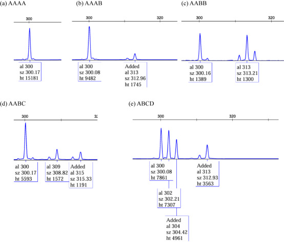
Nine polymorphic SSR loci were randomly chosen for validation using fluorescently labeled primers. Forward primers were labeled at the 5′ end with FAM, HEX, or ROX fluorophores. The PCR products were preliminarily validated via 2% agarose gel electrophoresis and subsequently purified for capillary electrophoresis, which was performed by Beijing Qingke Biotechnology Co., Ltd. Genotyping was conducted using fluorescence-based detection and analyzed with GeneMarker (v1.75; https://softgenetics.com/products/genemarker/). Given that P. pingi is a tetraploid species (4n = 98), manual curation was essential to ensure accurate genotype calling. Since automatic allele calling by the software may only record one or two alleles based on peak numbers, manual interpretation of allele counts and peak intensity ratios was implemented to refine genotyping (Fig. S1).
2.3.4. Genetic diversity analysis of SSR loci
Genetic diversity analyses were conducted on the validated SSR loci. The Shannon diversity index (I) was calculated using ATetra, whereas other parameters were calculated using GenoDive (v3.0), which supports polyploid data. The metrics analyzed included the number of alleles (Na), allele frequency (AF), the effective number of alleles (Ne), expected heterozygosity (He), observed heterozygosities (Ho), and Hardy–Weinberg equilibrium (HWE). Furthermore, polymorphism information content (PIC) and observed heterozygosity (Ho) were computed using standard formulas.
PIC was calculated as follows:
PIC=1−n∑i=1p2i−2[n−1∑i=1n∑j=i+1p2ip2j]
Where n is the total number of observed alleles at the locus, and pi and pj represent the frequencies of the ith and jth alleles, respectively. According to the classification criteria, an SSR locus is considered highly polymorphic when PIC > 0.5, moderately polymorphic when 0.25 < PIC < 0.5, and lowly polymorphic when PIC < 0.25.
Observed heterozygosity (Ho) was calculated as:
Ho=Number of observed heterozygous individualsTotal number of individuals
2.4. Parentage identification
The validation of the nine SSR loci was conducted using 300 offspring from single-pair families and 270 offspring from the mixed-rearing group, following the procedures outlined in Section 2.4.3. The genotype data of the 12 parents and 570 offspring were then combined to calculate the genetic diversity parameters of the parental and offspring populations, including I、Na、AF、Ne、He、HWE、PIC, and Ho.
To assess the accuracy of parentage assignment, we conducted computer simulations using the FaMoz software.13 The cumulative probability of exclusion (CPE) was calculated based on allele frequency data for each SSR locus (Table S7), with markers treated as codominant. The exclusion probability (EP) for individual SSR loci and the CPE across multiple loci were computed using the “Exclusion Probabilities” module under the “Probabilities” submenu. Parentage assignment was subsequently performed using both Cervus (v3.0) and PAPA (v2.0), which infer parent-offspring relationships based on exclusion principles. All 300 single-pair family offspring and 270 offspring from the mixed-rearing rearing group were analyzed with both programs to ensure robust identification under varying rearing conditions. In Cervus, simulations were conducted under the assumption that both maternal and paternal genotypes were known, with a confidence level set at 95%. In PAPA, analysis was performed using a uniform error model with a total error rate of 0.02. Offspring were assigned to their most likely parents only when consistent matches were identified by both Cervus and PAPA; these concordant results were considered true parent-offspring pairs.
2.5. Analysis of genetic distance among parental individuals.
To evaluate the genetic distances among parental individuals, we employed the R packages poppr and adegenet. The raw SSR genotype data, comprising nine loci with four alleles per individual, were initially formatted by combining alleles at each locus into a hyphen-separated string (e.g., “16/26/28/30”). Subsequently, these formatted genotypes were transformed into a genind object using the df2genind function in adegenet, with ploidy explicitly set to four to account for the tetraploid nature of the individuals.
We applied the recode_polyploids function in poppr to standardize polyploid data prior to distance computation. Bruvo’s genetic distance was then calculated using the bruvo.dist function, specifying the repeat length of each locus based on the SSR motif (di-, tri-, or tetra-nucleotide repeats). Bruvo’s genetic distance ranges from 0 (indicating high genetic similarity) to 1 (indicating greater genetic divergence).
Correlation analyses were performed using the ggpubr package, and linear regression equations were generated using ggpmisc. All visualizations were created with ggplot2.
2.6. Estimation of genetic parameters for growth traits
A total of 270 individuals from the mixed-rearing groups of P. pingi were measured for three growth traits: TL, BL, and BW. For detailed analysis, parentage identification results and corresponding growth trait data of each family were compiled into an Excel spreadsheet. Normality tests of all offspring growth data were performed using the Kolmogorov–Smirnov (K-S) test in SPSS (v.23.0). Basic descriptive statistics, including mean, standard deviation (SD), maximum, and minimum values, were computed. Additionally, the coefficient of variation (CV) was calculated in Excel using the following formula:
CV=SDMean∗100%
Genetic parameters and breeding values (BLUPs) were estimated using ASReml 3.0 software (https://vsni.co.uk/software/asreml-r/). The estimation was conducted via an animal model, utilizing the restricted maximum likelihood (REML) method for variance component estimation and the best linear unbiased prediction (BLUP) approach for breeding value estimation.
The animal model applied in this study is as follows:
Yijk=μ+fijk+aijk+eijk
Where i, j, and k represent the sire, dam, and individual ID, respectively. Yijk is the observed phenotypic value of the trait; μ is the overall population mean; fijk represents the family effect (including common environmental effects); aijk is the additive genetic effect; and eijk is the random residual. Among these, μ and fijk were treated as fixed effects, while the others were treated as random effects. All random effects were assumed to follow a normal distribution and to be mutually independent.
Narrow-sense heritability (h2) was estimated using the nvpredict function in ASReml 3.0, based on the following formula:
h2=σ2aσ2a+σ2e
Where h2 is heritability, σa2is the additive genetic variance, and σe2 is the residual (phenotypic) variance. In general, traits with ℎ² values less than 0.1 are considered to have low heritability, those with 0.1 ≤ ℎ2 ≤ 0.3 exhibit moderate heritability, and values greater than 0.3 indicate high heritability.14
Genetic and phenotypic correlations between traits were estimated, using standard covariance-based formulas in ASReml 3.0:
rG=COVGXY√σ2GXσ2GY
rG=COVPXY√σ2PXσ2PY
Where rG and rP represent the genetic and phenotypic correlations between traits X and Y, respectively. COVGXY and COVPXY are the genetic and phenotypic covariance components between the two traits, and σG2, σP2 are the corresponding variances.
Results
3.1. Screening of polymorphic microsatellites
A total of 30,147 sequences harboring SSR loci were detected in the full-length transcriptome data. Using SSREnricher software, 548 potentially polymorphic SSRs were identified. From these, 50 SSR loci were randomly selected for polymorphism assessment. Among them, 22 primer pairs produced clear and well-defined amplification bands (Table S8). Subsequent analysis using non-denaturing PAGE confirmed polymorphism at 14 of these loci, evaluating the level of polymorphism of these primers in parents. Ultimately, nine highly specific and efficient SSR markers were validated using fluorescent capillary electrophoresis (Table 1).
All nine SSR loci demonstrated high levels of polymorphism among the 12 parental individuals, with PIC values exceeding 0.5 (Table S9).
3.2. Parentage identification system
Genetic diversity analysis of the P. pingi parental individuals and their F1 offspring revealed a total of 65 alleles across the 12 parents and 570 offspring at the nine SSR loci. The mean Na was 7.222, while the average Ne was 3.503. The mean Ho was 0.936, while the He averaged 0.692. The average PIC was 0.647, with all loci—except PP021 and PP001—showing PIC values above 0.5, indicating high levels of polymorphism. The mean I was 1.407. HWE analysis indicated that only loci PP021 and PP047 conformed to HWE expectations; all other loci showed significant deviations (Table 2).
Based on simulations conducted using FaMoz, the results indicated that in the absence of known parental genotypes, the exclusion probability per locus (E-PP) ranged from 0.480 to 0.771, with an average of 0.696, reflecting strong power to exclude non-parental assignments (Table S10). The cumulative probability of exclusion (CPE-PP) across all nine SSR markers reached 0.999984, which exceeds the recommended threshold of 0.9999 for reliable parentage identification (Fig. 2).

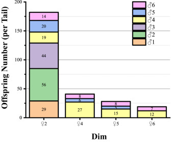
Among the 300 offspring from single-pair families, 288 individuals (96%) were assigned to the same parental pairs by both Cervus and PAPA, confirming the high accuracy of the combined parentage identification approach. Based on the established parentage identification system, the results from the mixed-rearing groups indicated that the dam ♀2 exhibited higher reproductive efficiency when crossed with these sires (Fig. S2).
3.3. Relationship between parental genetic distance and offspring growth
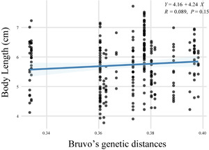
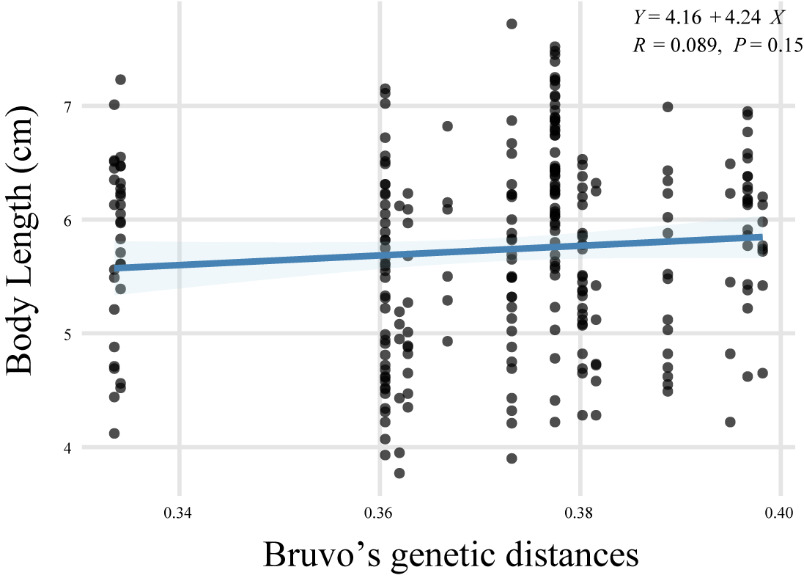
Bruvo’s genetic distances among parental individuals ranged from 0.33 to 0.40, with a mean of 0.37 (Table S11). Based on parentage assignments derived from the mixed-rearing group, we estimated the growth rates of offspring from different families. A linear regression analysis conducted between parental genetic distance and offspring growth rate resulted in the equation: Y = 4.16 + 4.24X (R = 0.089, P = 0.15) (Fig. 3), which indicates no statistically significant relationship between the two variables.
3.4. Genetic analysis of growth traits
K–S tests confirmed that all three traits followed a normal distribution, meeting the assumptions required for subsequent statistical analyses. The CV indicated differing levels of phenotypic variation among the traits. Body weight exhibited the highest variation (CV = 24.41%), significantly greater than that of total length (CV = 9.71%) and body length (CV = 10.51%) (Table S12).
Heritability estimates based on univariate animal models are presented in Table 3. The heritability of TL was 0.488 ± 0.119, indicating that 48.8% of the phenotypic variance in TL is attributable to additive genetic effects. BL had a heritability of 0.234 ± 0.072, while BW showed a heritability of 0.219 ± 0.069. According to standard classification criteria, TL is considered a trait with high heritability, whereas BL and BW fall into the moderate heritability category. In the multivariate animal model (Table 4), heritability estimates changed notably. The heritability of TL decreased to 0.171 ± 0.033, while body length remained similar at 0.210 ± 0.050. Interestingly, the heritability of body weight increased to 0.307 ± 0.082. Under the multivariate animal model, the heritability of BW is categorized as a high-heritability trait. In contrast, the heritability estimates for TL and BL remained within the moderate heritability range.
Genetic and phenotypic correlations among TL, BL, and BW were analyzed (Table S13). At the genetic level, the highest correlation was observed between TL and BL (0.976 ± 0.003), followed by TL and BW (0.935 ± 0.009), and BL and BW (0.933 ± 0.011). At the phenotypic level, TL and BL exhibited the strongest correlation (0.988 ± 0.016), followed by TL and BW (0.965 ± 0.050), and BL and BW (0.921 ± 0.080). All pairwise correlations were statistically significant (P < 0.05).
Discussion
4.1. Methods for the identification of SSR loci
Although the genomes of numerous economically significant aquaculture species have been sequenced, genomic resources for many endangered fish species remain limited. Consequently, transcriptome sequencing has emerged as a primary method for generating extensive sequence information and developing polymorphic SSR markers in these species. Third-generation full-length transcriptome sequencing provides the advantage of long read lengths, enabling the direct acquisition of complete mRNA sequences and structural information without the need for cDNA fragmentation or assembly. This approach has become a critical strategy for developing polymorphic SSR markers based on transcriptome data.15 In our study, a total of 58,021 unigenes were obtained, and SSR loci were identified in 30,147 unigenes, resulting in an SSR occurrence frequency of 51.96%. This frequency is significantly higher than that reported in many other fish species, such as Patagonian toothfish Dissostichus eleginoides (Smitt, 1898) (30.46%),16 indicating that third-generation transcriptome sequencing is a more effective approach than traditional transcriptome sequencing for the development of SSR markers. In this study, we employed the SSREnricher software to mine polymorphic loci across P. pingi populations from multiple geographic locations. As a result, the polymorphic SSR loci identified here may exhibit broader applicability. This is particularly important because previous studies have indicated that parentage identification systems developed from samples of limited geographic origin may compromise accuracy.7
4.2. Screening of polymorphic SSR loci in P. pingi
Among the 50 designed SSR primer pairs, 14 were successfully amplified and exhibited clear polymorphism. By integrating second- and third-generation sequencing data using SSREnricher, we identified that 63.64% of the 22 selected clear bands contained polymorphic SSRs. According to Luo et al.,12 over 90% of markers predicted by SSREnricher as polymorphic are indeed polymorphic in practice. However, it is evident that the probability of detecting polymorphic SSRs decreases in polyploid species. A similar phenomenon was reported in loach Misgurnus anguillicaudatus (Cantor, 1842), where only 24.44% of loci that were polymorphic in diploids remained highly polymorphic in tetraploids.17 One possible explanation is that, in polyploids, some alleles may fail to amplify due to mutations at primer-binding sites, leading to an underestimation of allele numbers.
A more critical consideration in the screening of polymorphic SSRs is determining the minimum number of loci required to construct a reliable parentage identification system. Based on our literature review, most studies suggest that at least seven polymorphic loci are necessary to achieve sufficient accuracy for parentage assignment.18,19 Notably, Wang et al.19 demonstrated that a set of 12 polymorphic loci could support the establishment of two independent parentage identification systems. Therefore, selecting at least eight highly polymorphic loci is considered a prudent and effective strategy. When more than 12 loci are available, constructing multiple complementary parentage identification panels becomes feasible.
4.3. Establishment of a parentage assignment system
To establish a reliable parentage identification system, we first evaluated key indicators of population genetic diversity, including Na, Ne, I, Ho, He, and PIC. A total of 65 alleles were detected across both the parent and offspring populations, with an average of 7.222 alleles per locus and an average Ne of 3.503. The mean Ho was 0.936, and the He was 0.692, indicating a high level of genetic diversity in the population. The average PIC value was 0.647, with all except PP021 (0.475) and PP001 (0.473)-exceeding 0.5, demonstrating that the majority of loci were highly polymorphic. The average I was 1.407, further supporting the conclusion of substantial genetic diversity. Overall, the genetic diversity parameters of the nine SSR loci used in this study indicate that P. pingi populations harbor sufficient variation, making these markers suitable for constructing a robust parentage identification system.
The PIC is a critical parameter for evaluating the effectiveness of parentage identification systems. Typically, SSR loci with a PIC value greater than 0.5 suggest the presence of multiple alleles with relatively even frequency distributions, which is advantageous for individual identification and accurate parentage assignment. In this study, two loci exhibited PIC values slightly below 0.5, specifically 0.475 and 0.473. However, a previous study suggested that loci with PIC values above 0.4 may still be informative and useful for parentage analysis.20 Subsequent validation confirmed that these two loci were indeed effective in the parentage identification system. Nonetheless, we do not recommend the inclusion of loci with PIC values lower than 0.5, as the initial validation involving 12 parental individuals demonstrated that all selected loci exhibited PIC values exceeding 0.5. Surprisingly, our study demonstrated that the majority of microsatellite loci adhered to HWE. Napora-Rutkowski et al.21 noted that deviations from HWE are relatively common in captive fish populations, primarily attributed to hatchery practices involving a limited number of founder individuals and unbalanced sex ratios. A comparable observation was made by Sánchez-Velásquez et al.,5 where eight out of 10 polymorphic loci showed deviations from HWE. However, in their study, the influence of inbreeding was excluded due to the use of wild populations, and a high frequency of null alleles (Null Freq) was identified as a significant contributing factor. In contrast, inbreeding is likely a critical factor contributing to the observed deviations in our study. It is also essential to evaluate whether deviations from HWE could compromise the accuracy of the parentage identification system. Theoretically, HWE deviations may alter allele frequency estimates, thereby reducing the statistical confidence of parentage assignment. Nevertheless, in systems utilizing multiple polymorphic markers, the impact of HWE deviations appears to be negligible.5 Consequently, rather than focusing exclusively on HWE status, greater emphasis should be placed to the PIC of each locus. Extensive research has highlighted that low PIC values can elevate the risk of misassignment and increase analytical cost, whereas the influence of HWE deviations on parentage analysis remains generally limited.5,20
Using nine highly polymorphic SSR loci, we conducted parentage analysis on 12 candidate parents and 300 offspring individuals from single-pair families. The combined CPE reached 0.999984, corresponding to a simulated accuracy of 99.99%, which significantly exceeds the threshold for confirmed parentage (≥ 99.73%). In this study, the actual assignment accuracy for single-family P. pingi offspring was 96%, slightly lower than the simulated value but still sufficiently high for practical applications. In other studies, parentage accuracy based on 12 highly polymorphic loci reached 100% in mixed-family settings, with an accuracy of 98.69% in the test population. In grass carp Ctenopharyngodon idella (Valenciennes, 1844), 12 microsatellite loci were optimized into three multiplex PCR systems for parentage identification, and 99.6% of offspring were successfully assigned to a specific parental pair.22 These findings demonstrate the feasibility of using diploid analysis software, such as Cervus v3.0 and PAPA, to infer parentage even in polyploid fish species.
4.4. Genetic distance analysis and its relationship with offspring growth
Regulating the genetic distance between breeding pairs can significantly enhance offspring survival and average BL.3 A low genetic distance increases the likelihood of inbreeding depression, which can lead to reduced fitness and viability of the offspring. A study demonstrated that wild populations with greater genetic distances exhibited significantly higher growth rates compared to cultured populations with smaller genetic distances.23 This highlights the importance of maintaining an effective breeding population by selecting parent pairs with moderate to high genetic divergence. In this study, no definitive results were obtained, as the positive correlation between growth traits and genetic distance was not statistically significant. This may primarily result from the relatively narrow genetic background of the broodstock, which limited the overall range of genetic divergence and reduced the statistical power to detect associations. In addition, the sample size of breeding pairs was relatively small, which may have weakened the robustness of the correlation analysis. Moreover, the relationship between genetic distance and heterosis is likely non-linear, with both insufficient and excessive genetic divergence potentially leading to suboptimal offspring growth. Non-additive genetic effects and environmental factors may also obscure the true genetic relationship between parental distance and offspring growth.
4.5. Heritability and breeding value evaluation
In genetic breeding of aquatic animals, the heritability of growth traits serves as a critical indicator for evaluating the degree to which phenotypic variation is influenced by genetic factors. A higher heritability suggests a greater genetic contribution to trait variation, thereby indicating stronger potential for genetic improvement via selective breeding. In this study, the estimated heritability of growth traits in P. pingi exhibited differences between the univariate and multivariate models. Specifically, under the univariate model, the heritability estimates were 0.488 ± 0.119 for TL, 0.234 ± 0.072 for BL, and 0.219 ± 0.069 for BW. Conversely, under the multivariate model, the heritability estimates were 0.171 ± 0.033 for TL, 0.210 ± 0.050 for BL, and 0.307 ± 0.082 for BW. Similarly, previous studies on Asian seabass Lates calcarifer (Bloch, 1790) reported heritability estimates ranging from 0.11 – 0.32 for BL and 0.12 – 0.34 for BW, which align within a comparable range.24 These findings underscore significant discrepancies in heritability estimates for TL and BL between the two models, while the heritability of BW increased in the multivariate model. Such inconsistencies may arise due to genetic correlations among traits. The multivariate model incorporates covariance structures between traits, potentially enhancing the accuracy of heritability estimates, particularly for traits with low individual heritability or strong genetic correlations. Further analysis of both genetic and phenotypic correlations among TL, BL, and BW revealed values exceeding 0.9 (P < 0.05), indicating robust intertrait relationships. Consequently, the multivariate approach is deemed more suitable for this study. Notably, BW emerged as a trait of high breeding relevance and could serve as a key target in future selection programs. In general, traits with high heritability can be effectively improved through mass selection, whereas those with low heritability necessitate family-based selection strategies to achieve enhanced breeding efficiency.
In practical terms, the developed parentage identification system enables mixed-family communal rearing with reliable pedigree reconstruction (>95–99% assignment), which is essential for estimating individual EBVs under BLUP/GBLUP, implementing factorial matings, and running selection in commercial settings. By linking growth phenotypes to reconstructed pedigrees, breeders can rank broodstock on EBVs for BW (the most promising target in this study) while constraining coancestry to control inbreeding and maintain effective population size across generations. Nevertheless, the current work is limited by the moderate sample size and potential environmental influences on growth traits. Future studies integrating larger breeding populations, multi-generation validation, and genomic datasets will further enhance the accuracy and applicability of the developed system.
Acknowledgments
Individuals other than authors can be acknowledged by a brief statement immediately following the text. Acknowledgments of grant support should also be placed here.
Authors’ Contribution
Conceptualization: Siyi Zhu (Equal), Wei Luo (Equal), Zongjun Du (Equal). Formal Analysis: Siyi Zhu (Equal), Xing Ying (Equal), Wei Luo (Equal). Investigation: Siyi Zhu (Equal), Longjun Deng (Equal), Tiancai Li (Equal), Tong Li (Equal), Qingjie Wang (Equal), Shun Zhong (Equal), Xing Ying (Equal), Fulin Dai (Equal), Dongjie Wang (Equal). Validation: Siyi Zhu (Equal). Writing – original draft: Siyi Zhu (Equal), Wei Luo (Equal). Methodology: Dongjie Wang (Equal), Wei Luo (Equal), Zongjun Du (Equal). Funding acquisition: Wei Luo (Equal), Zongjun Du (Equal). Project administration: Wei Luo (Equal), Zongjun Du (Equal). Writing – review & editing: Wei Luo (Equal), Zongjun Du (Equal). Data curation: Zongjun Du (Lead).
Competing of Interest – COPE
The authors declare there are no competing interests.
Ethical Conduct Approval – IACUC
All experimental protocols in this study were approved by the Animal Research and Ethics Committee of Sichuan Agricultural University (SAU20230310). Fish treatments were conducted in accordance with the guidelines for the Care and Use of Agricultural Animals in Research and Teaching, authorized by the Science and Technology Bureau of China. Approval from the Department of Wildlife Administration was not required for the experiments described in this paper.
Informed Consent Statement
All authors and institutions have confirmed this manuscript for publication.
Data Availability Statement
The transcriptome sequence data supporting the findings of this study are publicly available in the National Genomics Data Center (https://ngdc.cncb.ac.cn/gsa/) under accession numbers CRA016173 and CRA024585.
Funding
This work was supported by the National Natural Science Foundation of China (No. 32172998), the Yalong River Percocypris pingi Germplasm Characterization and Its Application in Artificial Propagation Project (No. 000023-22XB0141), the National Modern Agricultural Industry Technology System – Sichuan Innovation Team (No. SCCXTD-2025-15), and the Study and Demonstration on the Breeding of New Cobitidae Varieties and Standardized Aquaculture Techniques Project (No. 2021YFYZ0015).