Temperature effects on mariculture output in China: Evidence from causal forest analysis

Introduction

The marine system is continuously affected by global warming. According to the Intergovernmental Panel on Climate Change (IPCC) Sixth Assessment Report (AR6), global near-surface sea surface temperature (SST) shows a significant upward trend, and the frequency and intensity of extreme heatwave events are both increasing.¹ As a sensitive and significantly affected area of climate change, China frequently experiences high-temperature heatwaves in coastal regions.² Studies have pointed out that climate change may have adverse effects on the marine ecological environment and fish communities,^3–5 which brings multi-dimensional challenges to China’s mariculture industry. The Food and Agriculture Organization (FAO) of the United Nations has also repeatedly emphasized in the “The State of World Fisheries and Aquaculture” report that climate risks have become one of the greatest challenges to the sustainable development of global aquaculture.⁶

As a major maritime and fishery country, China has always adhered to the development policy of focusing on aquaculture in the fishery sector. Mariculture is an important marine pillar industry in China, playing a major role in ensuring food security and driving economic development in coastal areas. China’s mariculture species composition is rich, mainly covering five major categories: fish, shrimp, crab, shellfish, and algae. Among them, shellfish (such as oysters and scallops) and algae (such as kelp and laver) account for the vast majority of the output, while high-economic-value fish (such as large yellow croaker and grouper) are mostly cultured in deep-water cages or offshore ponds. Because different species have different physiological tolerance ranges to temperature, and the physical environments of culture systems (such as deep-water cages and offshore ponds) are different, the impact of temperature rise on output has complex species specificity and system specificity.^7,8

Therefore, an in-depth analysis of the impact of global warming on the mariculture industry has important practical significance. Taking 10 coastal provinces and municipalities across the country as the research object and using panel data from 2010 to 2023, this paper comprehensively considers multiple influencing factors such as capital and labor input, marine environment, regional development level, and technological input. It uses the causal forest model to identify the causal effect of temperature rise on mariculture output, and further examines the differences in treatment effects of temperature rise on mariculture output under different conditions. This paper studies the following three questions: Does temperature rise affect mariculture output? Is there a marginal pattern in the impact of temperature rise on mariculture output? Is the degree of impact of temperature rise on mariculture moderated by covariates?

Literature Review

Research related to global warming and the mariculture industry can be divided into three categories.

The first is to explore the impact of climate warming on the marine ecological environment. Some scholars believe that temperature rise will lead to an increase in marine salinity, elevated oxygen content, seawater acidification, and frequent marine disasters, thereby affecting the physiological processes of marine organisms. This may make the original mariculture species no longer suitable for culturing, thus affecting fishery output. Hollowed et al.⁹ predicted the impact of climate change on marine biological communities, suggesting that climate change may cause a 30-60% decline in potential fish production, and China’s coast will be one of the most severely warmed areas, but the overall decline in fish biomass density is not large. Jennings S et al. (2010) sampled and investigated the population distribution of 36 fish species in the North Atlantic, finding that for every 1°C increase in average water temperature, the investigated fish populations would move 0.5-0.8 degrees towards the poles. Sarmiento J et al. (2004) used 6 coupled climate simulation models to study the impact of climate warming on marine organisms, and found that the contraction or expansion of regional biomes at different dimensions and productivity levels also differs. From the perspective of biological mechanisms, temperature rise interferes with mariculture output through multiple pathways. The first is physiological stress: when the ambient temperature exceeds the thermal tolerance limit of the species, it will lead to growth retardation, metabolic imbalance, and even massive mortality. Elevated temperatures not only reduce the dissolved oxygen content of seawater, but also increase the basal metabolic rate of poikilotherms, thereby inducing oxygen stress in aquatic animals. The second is pathological risk: climate warming favors the breeding and spread of pathogens such as Vibrio, significantly increasing the disease outbreak rate in aquaculture.

The second is to study the performance of marine fisheries under climate change. Some scholars believe that climate change will lead to a decrease in fishery output, and this impact effect presents regional differences. Froehlich et al.¹⁰ evaluated the vulnerability of global marine aquaculture to climate change, suggesting that Southeast Asia and coastal China are among the regions most severely threatened by heat stress. The study by Ahmed et al.¹¹ further pointed out that the impact of temperature fluctuations on open pond culture is significantly higher than that on closed or offshore deep-water culture systems, reflecting the system-specific differences of climate impacts. Ding (2017) evaluated the vulnerability of fisheries to climate change at the national level, and found that the fishery industries in countries with sound governance and longer life expectancy have stronger coping capabilities to climate change. Blasiak et al.¹² studied the impact of climate change on marine fisheries, and found that underdeveloped countries showed stronger vulnerability when facing climate change.

The third is to study the specific factors affecting the mariculture industry. In the field of research on mariculture production efficiency, efficiency evaluation methods have been widely applied. An evaluation combining the SBM-DEA model with undesirable outputs and the meta-frontier analysis framework shows that there is significant technological heterogeneity in the ecological efficiency of mariculture in China’s coastal areas, and the input-output relationship tends to be complicated. Market demand, technological promotion, and equipment input are the main factors driving mariculture output and the structural adjustment of cultured varieties. From the perspective of total factor productivity, the growth of production efficiency in the mariculture industry is mainly driven by technological progress, and adaptive management strategies are also key to mitigating the negative impacts of climate warming on fisheries. In addition, the annual average ecological efficiency of China’s mariculture is generally low, and insufficient technological level is the core factor restricting efficiency improvement.

Existing studies show that climate change may have a negative impact on mariculture output, and this impact exhibits large heterogeneity across different regions. In addition, mariculture output is also affected by multiple factors such as technological level. There is also a close coupling relationship among temperature rise, ecological environment changes, and fishery output. However, existing literature has not sufficiently identified the sources of heterogeneity, while the causal forest model can better solve this problem.

Currently, methods combining machine learning with causal inference are gradually emerging in the field of agricultural and resource economics. Especially when evaluating climate change or policy shocks, machine learning algorithms represented by the causal forest have shown great advantages in breaking through the limitations of traditional econometric models, identifying complex influencing factors, and determining heterogeneous treatment effects.

Therefore, the contributions of this paper are: First, in terms of research perspective, it comprehensively considers multiple factors such as marine environment, technological input, and regional development level to evaluate the impact of climate warming on mariculture output. Second, in terms of research methods, it selects the causal forest model to identify the impact of temperature rise on mariculture output, expanding the application scenarios of this model to a certain extent. Third, in terms of research content, utilizing the causal forest model’s advantage in capturing heterogeneous effects, this paper examines the differences in treatment effects of climate warming on mariculture output among groups with different characteristics.

Materials and Methods

Research Method

The Random Forest algorithm, proposed by Breiman,¹³ is a machine learning model known for its strong predictive capabilities. The model constructs multiple decision trees \(\{ h\left( x,\Theta_{k} \right),k = 1\ldots\}\) through bootstrap sampling from training data, where each tree independently predicts the data. Through k rounds of training, a sequence of classification models \(\{ h_{1},h_{2},\ldots,h_{k}\}\) is generated. The final prediction is the arithmetic mean of the predictions from each decision tree.

The Causal Forest algorithm, proposed by Wager and Athey¹⁴ based on Generalized Random Forests, is a method that focuses on estimating treatment effects at the individual level, making it particularly effective for addressing heterogeneity in causal relationships. The Causal Forest model incorporates Random Forests as an Adaptive Kernel Method into a partial linear regression model. It estimates the Conditional Average Treatment Effect (CATE), denoted as \(\tau(x)\), for each individual, ultimately obtaining the estimation of the average treatment effect (ATE):

\(\widehat{\tau}(x) = \frac{\frac{1}{n}\sum_{i = 1}^{n}{\alpha_{i}(x)(Y_{i} - {\widehat{m}}^{( - i)}\left( X_{i} \right))(W_{i} - {\widehat{e}}^{( - i)}\left( X_{i} \right))}}{\frac{1}{n}\sum_{i = 1}^{n}{\alpha_{i}(x)}{(W_{i} - {\widehat{e}}^{( - i)}\left( X_{i} \right))}^{2}}\)

Where \(W\) represents the treatment variable (regional temperature in this study); \(Y\) represents the outcome variable (mariculture output); \(X_{i}\) represents the covariates; \(\ \widehat{m}\left( X_{i} \right)\) is the predicted value given the covariates; \(\widehat{e}\left( X_{i} \right)\) is the probability of individual i receiving the treatment given the covariates; and \(\alpha_{i}(x)\) is the adaptive kernel function. This study utilized the causal_forest package in R to perform the estimation.

Data Sources and Variable Description

In the selection of research samples, because Shanghai only has mariculture output in very few years and the output is small, data from 10 coastal provinces (Liaoning, Tianjin, Hebei, Shandong, Jiangsu, Zhejiang, Fujian, Guangdong, Guangxi, and Hainan) from 2010 to 2023 were selected for the study. The variables include three categories: treatment variable, outcome variable, and covariates.

The outcome variable is mariculture output, and the data is compiled from the “China Fishery Statistical Yearbook”.

In the selection of the treatment variable, this paper uses sea surface temperature as a proxy variable for regional temperature. SST data are derived from the monthly gridded high-precision climate dataset provided by the Physical Sciences Laboratory (PSL) of the National Oceanic and Atmospheric Administration (NOAA). In the specific data processing workflow, using the spatial data processing module of the R language, the global SST raster data was spatially cropped according to the latitude and longitude boundaries (Bounding Box) of the offshore waters of the 10 coastal provinces in China. By removing land grids and extracting the monthly mean values of all marine grid points within the exclusive sea areas of each province, the annual sea surface temperature panel data for each province from 2010 to 2023 was finally calculated through aggregate averaging.

In terms of covariate selection, the inputs of labor, capital, resources, and technology factors may affect mariculture output. Therefore, the number of professional practitioners in the mariculture industry is selected to measure labor factor input.

In terms of capital input, the proportion of factory farming area to the total farming area and the total tonnage of marine motorized fishing vessels are selected. Generally speaking, a higher proportion of factory farming area means a higher degree of mechanization in fishery production and a larger proportion of capital input. Productive fishing vessels specifically serving the mariculture segment are capital-type input factors that directly affect fishery output.

In terms of resource input, fingerling input is the foundation of culture output, so the amount of mariculture fingerling input (tens of thousands) is selected to measure resource input.

Studies by Ding Q (2017) and others show that structural factors are also important factors affecting fishery output. Therefore, per capita GDP is selected to measure the level of regional economic development, and regional population is selected to represent market size.

Temperature rise has a great impact on the marine ecological environment, and the ecological environment may also affect culture output. Therefore, the excellent rate of nearshore water quality and the area of regional marine protected areas are selected to measure the marine ecological environment of a certain region. In addition, existing studies emphasize that the degree of impact of climate change on aquaculture depends on the moderation of local institutions and governance capabilities. Fishery administration agencies can provide administrative management and service guidance for fishery production by implementing fishery regulations and standardizing culture behaviors. Therefore, this paper selects the number of fishery administration agencies to measure the fishery governance capability of a certain region.

Natural disasters are important shocks causing fluctuations in mariculture output. Disaster events such as high-temperature heatwaves, storm surges, and red tides will directly lead to the death of cultured organisms and the destruction of culture facilities, resulting in irreversible output losses. Therefore, the percentage of aquatic product loss caused by fishery disasters to the fishery output value is selected as a proxy variable for risk shocks to control the impact of natural disasters on mariculture output.

Covariate data are sourced from the “China Fishery Statistical Yearbook”, the “China Marine Statistical Yearbook”, the “Bulletin of China’s Marine Ecological Environment”, and the National Bureau of Statistics.

Furthermore, to mitigate potential heteroscedasticity in the data, this study applied a natural logarithmic transformation to the following variables: mariculture output, mean sea surface temperature, number of professional mariculture practitioners, year-end possession of marine motorized fishing vessels used for mariculture, mariculture fingerling input, per capita GDP, regional population, total area of marine nature reserves, number of fishery administration agencies, and fishery technology promotion funds. This aligns the data distribution more closely with the normality assumption and converts the estimated coefficients into elasticities or semi-elasticities, thereby more intuitively reflecting the relative impact of changes in each variable on the output.

Results

Causal Identification Assumptions and Model Specification

Before conducting the causal forest estimation, two identification assumptions are discussed.

Unconfoundedness assumption. This study incorporates 11 dimensions of covariates, including labor input, capital input, resource input, regional economic development level, market size, ecological environment, governance capability, technological factors, and natural disasters, which largely mitigates the omitted variable bias.

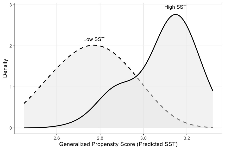
Common support assumption. We use the Generalized Propensity Score (GPS) method to test the common support assumption. A linear regression of sea surface temperature on the covariates is performed to obtain the predicted values (GPS), and the samples are divided into high and low groups based on the actual median temperature. Figure 1 shows the GPS density distributions for the high SST group and the low SST group. The results show that the common support interval for the two groups is [2.70, 3.03], and the overlap area ratio reaches 60.6%, indicating that different temperature levels have good overlap in the covariate space, satisfying the common support assumption under continuous treatment. Therefore, the estimation of the causal forest will not suffer from severe extrapolation bias due to a lack of common support.

Figure 1.Density plot of generalized propensity score

Estimation Results Based on the Causal Forest Model

All model estimations in this paper were completed in the R statistical computing environment (version 4.4.2). Based on the generalized random forest algorithm framework, this paper uses the grf package (version 2.6.1) for core measurements. In setting the specific package parameters, to balance estimation robustness and computational efficiency, this paper sets the minimum leaf node sample size (min.node.size) to 5. Meanwhile, to avoid the risk of overfitting, the honest estimation tree procedure was executed, with the split ratio set to 0.5. When performing causal forest estimation, the number of decision trees has a significant impact on model performance. Since this study uses annual panel data of 10 provinces, the data scale is relatively small, so the number of trees should not be too large. Table 2 shows the estimation results under the number of decision trees of 400, 450, 500, and 550. Taking 400 trees as an example, the ATE of temperature rise on mariculture output is -0.6237, with a standard error of 0.2706, which is significant at the 5% level. This indicates that for every 1% increase in sea surface temperature, mariculture output decreases by an average of about 0.62%. When the number of decision trees increases to 450, 500, and 550, the ATE stabilizes between -0.56 and -0.64, and all are significant, indicating that the model has good robustness.

Marginal Impact Pattern of Temperature Rise on Mariculture Output

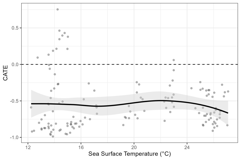
Figure 2 reports the distribution of the CATE of sea surface temperature on mariculture output with temperature changes. The results show that within the observation interval of 12°C-24°C, the negative effect of sea temperature rise on mariculture output generally remains stable, with the effect magnitude stabilizing in the range of -0.4 to -0.5, and there is no significant nonlinear fluctuation, indicating that the impact of normal temperature fluctuations on mariculture output is consistent. However, when the sea temperature exceeds 24°C, as the temperature rises, the negative inhibitory effect shows an increasing trend, indicating that extreme high temperatures may lead to damage to mariculture output. Across the entire temperature interval, the 95% confidence intervals of the treatment effects do not contain 0, indicating that the negative impact of sea temperature rise on mariculture output is universal, and the core conclusion is robust.

Figure 2.CATE of temperature rise on mariculture output

Variable Importance Analysis

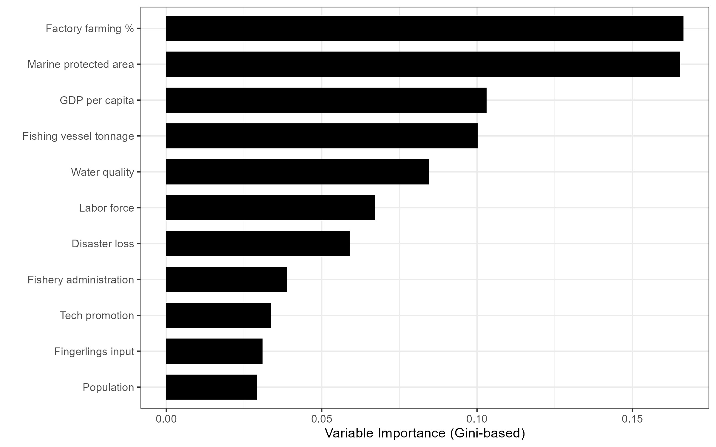
To identify the driving factors of the heterogeneity in the effect of sea temperature on mariculture output, this paper calculates the importance scores of each covariate using the Gini coefficient, and the results are shown in Figure 3. Among them, the proportion of factory farming and the area of marine protected areas have higher importance scores and are the core driving factors of heterogeneity, indicating that the industrialization level of culture models and the construction of marine ecological protection are key factors determining the ability of coastal areas to resist the impact of sea temperature rise. Per capita GDP and the tonnage of fishing vessels represent the important roles of regional economic development level and fishery industrial foundation. Basic production conditions such as nearshore water quality and labor force are moderate influencing factors, while the explanatory power of variables such as fishery administration and technology promotion is relatively weak.

Figure 3.Importance ranking of covariates affecting mariculture output

Individual Treatment Effects of Temperature Rise on the Mariculture Industry under Different Conditions

Treatment Effects at Different Regional Economic Development Levels

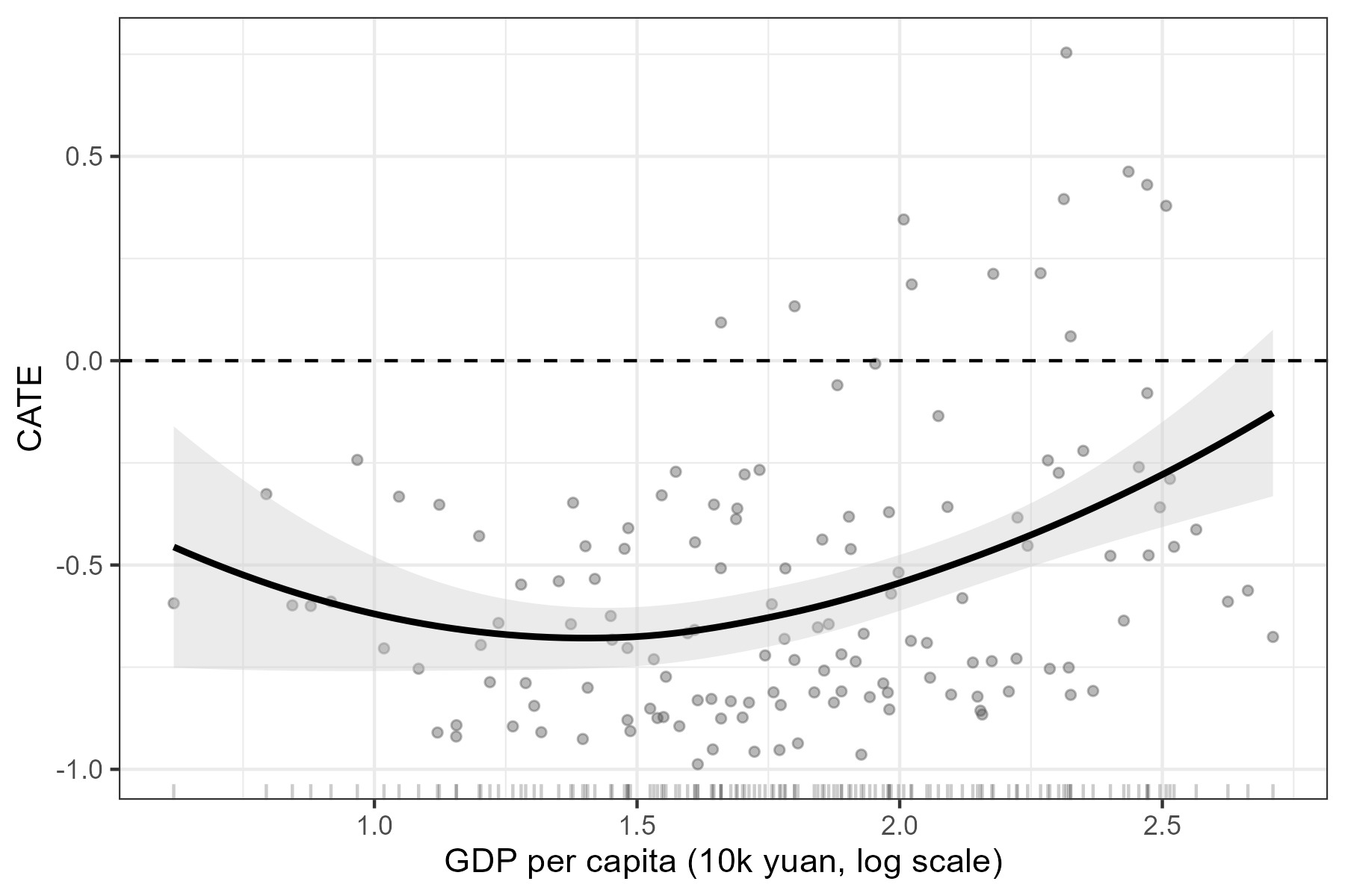
Figure 4 presents the variation trend of the CATE estimated based on the causal forest model with per capita GDP, primarily revealing the moderating characteristics of regional economic development level on sea temperature shocks. In the interval where the logarithmic value of per capita GDP is below 1.5, as the economic development level increases, the negative inhibitory effect of sea temperature rise on mariculture output continues to strengthen, reaching a peak when the logarithmic value of per capita GDP is in the range of 1.2-1.5, with the CATE dropping close to -0.7. This indicates that high-temperature shocks have a larger impact on coastal areas with a moderate level of economic development. However, after the logarithmic value of per capita GDP exceeds 1.5, as per capita GDP further increases, the negative effect of sea temperature continues to weaken. In the high development level interval where the logarithmic value of per capita GDP is above 2.5, the CATE has converged to a lower level. This result indicates that the hedging effect of economic development against climate risks exhibits a threshold effect. Middle-income regions have not yet completed the industrial upgrading of culture models and cannot effectively resist high-temperature shocks, while high-income regions can build a comprehensive risk resistance system through capital investment, technological iteration, and the promotion of factory farming.

Figure 4.Heterogeneous distribution of the effect of sea temperature on mariculture output under varying per capita GDP

Treatment Effects under Different Disaster Conditions

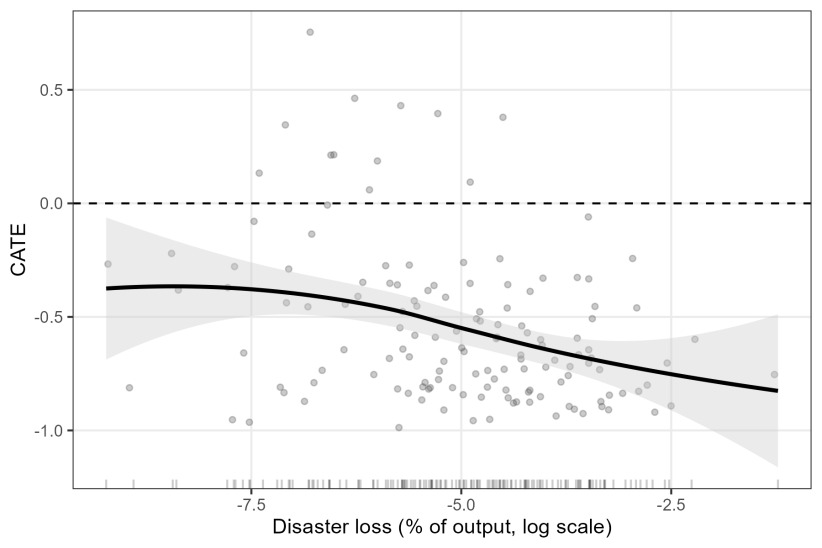
Figure 5 demonstrates the variation pattern of the sea temperature culture effect with fishery disaster losses. The results show that the negative inhibitory effect of sea temperature rise exhibits a linear increasing characteristic as the scale of disaster losses expands. As fishery disaster losses expand, the CATE curve continues to slope downward, the magnitude of the negative shock continues to widen, and the absolute value of the effect expands from around -0.3 to nearly -0.8. This finding reveals that in areas with higher fishery disaster risks, the risk-resistance capacity of culture production is weaker, and the high-temperature shocks brought by sea temperature rise will further amplify the negative impact on culture output. This result provides a basis for the construction of fishery disaster prevention and control systems in China’s coastal areas; disaster-prone areas are key zones for high-temperature climate risk prevention and control.

Figure 5.Heterogeneous distribution of the effect of sea temperature on mariculture output under varying fishery disasters

Treatment Effects under Different Fingerling Input Conditions

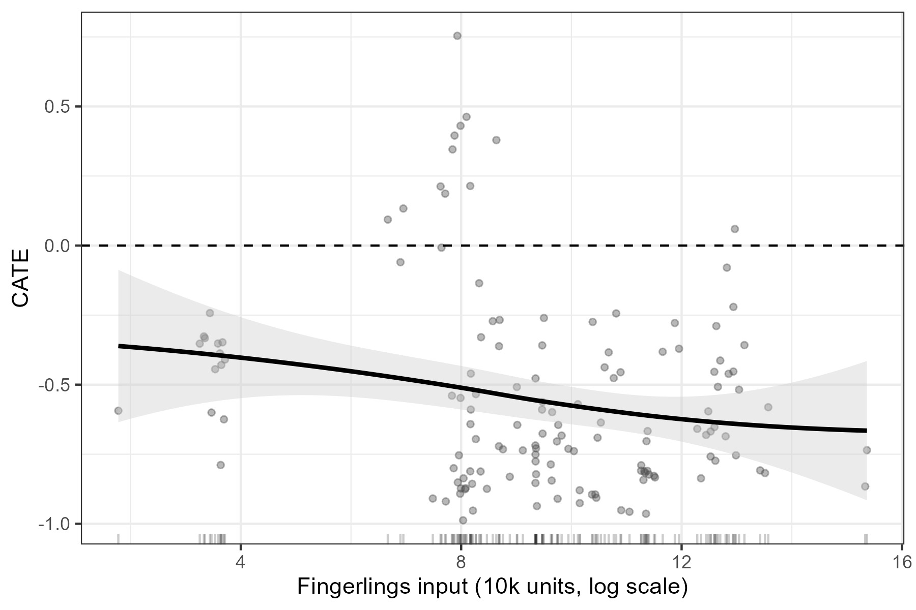
Figure 6 reports the moderating effect of fingerling input on the sea temperature culture effect. The results show that the negative inhibitory effect of sea temperature rise continuously strengthens as the scale of fingerling input expands. As the logarithmic value of the fingerling input scale increases from 4 to 16, the CATE curve continues to move downward, the negative effect expands from -0.3 to nearly -0.7, and the intensity of high-temperature shocks continuously increases. The scale of fingerling input corresponds to culture density and the scale level of production. The traditional extensive high-density culture model is significantly more sensitive to water temperature fluctuations. In a high-temperature environment, it is more prone to disease outbreaks and a decline in culture survival rates, thereby amplifying output losses. This result forms a contrast with the previously mentioned factory farming: an extensive development pattern that purely relies on expanding fingerling input to increase the culture scale will aggravate the exposure of mariculture to high-temperature climate risks, while intensive model upgrading centered on factory recirculating aquaculture is the important path to hedge against the negative impacts of climate change.

Figure 6.Heterogeneous distribution of the effect of sea temperature on mariculture output under varying fingerling input

Robustness Checks

Sensitivity Analysis (Unobserved Confounding)

To evaluate the potential impact of unobserved confounding on the estimation results, we adopt the method of Cinelli & Hazlett¹⁵ to conduct a sensitivity analysis. Using the level of fishery technology promotion (FishTechProm) as the benchmark, this paper simulates unobserved confounding scenarios with 1, 2, and 3 times the explanatory power of this variable, respectively, and calculates the adjusted ATE under different confounding intensities. The test results are shown in Table 3. The test results show that when the explanatory power of the unobserved confounding variable reaches 1, 2, and 3 times that of the fishery technology promotion level, the adjusted ATEs are -3.0711, -3.0438, and -3.0166, respectively, maintaining a negative sign consistent with the benchmark model. Meanwhile, the 90% confidence intervals of the adjusted effects under all confounding intensities do not contain 0, remaining statistically significant. According to the core criterion of the Oster test, even in the presence of an unobserved confounding variable with 3 times the explanatory power of the controlled core covariate, the research conclusion of this paper still holds, and it is almost impossible for potential unobserved confounders to overturn the estimation results of the benchmark model. The above tests fully prove that the core causal conclusions of this paper are robust to the problem of unobserved confounding, and the estimation results are reliable.

Placebo Test

To further rule out the interference of random factors and unobserved confounding variables on the core conclusions, this paper conducts an analysis using a placebo test.

This paper executed placebo simulations for 250, 500, and 1000 times, respectively, and the test results are shown in Table 4. The results show that regardless of the adjustment in the number of simulations, the mean placebo ATEs of the fictitious treatment variable stabilize around 0. Specifically, the mean placebo ATE for 500 simulations is only 0.0007, and the mean for 1000 simulations is -0.0042, showing almost no systematic bias; simultaneously, the 95% placebo ATE distribution intervals under all simulation counts contain the value 0, indicating no significant causal relationship between the fictitious treatment variable and mariculture output.

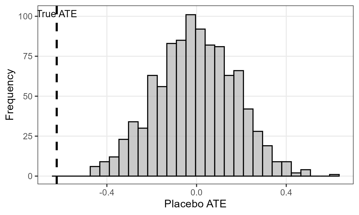
The histogram of the placebo ATE distribution for 1000 simulations is shown in Figure 7. From the distribution shape, the placebo ATE exhibits a normal distribution centered around 0, with the vast majority of simulated ATE values concentrated in the [-0.4, 0.4] interval; whereas the ATE of the true benchmark model in this paper is -0.6237, which falls in the left tail of the placebo distribution and is completely separated from the placebo distribution. None of the 1000 simulated placebo estimates are smaller than the true benchmark result.

Figure 7.Histogram of placebo ATE distribution for 1000 simulations

Discussion

Conclusions

Based on panel data of coastal provinces and municipalities in China, this paper uses the causal forest model to identify the causal effect of sea surface temperature rise on mariculture output. It verifies the robustness of the core results through an unobserved confounding bounds test and a placebo test, and systematically examines the heterogeneity characteristics and core driving factors of the effect. The main research conclusions are as follows:

First, sea surface temperature rise has a significant negative causal effect on mariculture output in China’s coastal areas. Under model specifications with different numbers of decision trees, the ATE of sea temperature rise stabilizes in the range of -0.56 to -0.64, and all are significant at the 5% statistical level, indicating that elevated sea temperatures exert an inhibitory effect on mariculture output.¹⁰ Variable importance ranking results show that the proportion of factory farming and the area of marine protected areas are the primary factors driving effect heterogeneity, while variables such as regional per capita GDP and fishery vessel scale are key to determining mariculture output levels and the capacity to resist climate risks.

Second, the impact of sea temperature rise on mariculture output presents non-linear threshold characteristics. Within the sea temperature range of 12°C to 24°C, the negative shock of temperature rise generally remains stable; when the sea temperature exceeds the critical value of 24°C, the negative inhibitory effect shows an increasing trend, indicating that extreme high temperatures are a key risk source for impaired mariculture output, and the higher the temperature in a region, the stronger the negative impact of sea temperature rise.⁷

Third, the moderating effect of regional economic development level on sea temperature shocks exhibits a U-shaped threshold characteristic. In lower per capita GDP intervals, the negative shock of sea temperature strengthens as the economic development level increases; coastal areas with a moderate economic development level are vulnerable groups to high-temperature shocks. When per capita GDP crosses the threshold value, regions with a high economic development level can effectively mitigate the negative impact of sea temperature rise through technological iteration and culture model upgrading.¹²

Fourth, culture production conditions significantly amplify the impact of high-temperature shocks. The larger the scale of fishery disaster losses in a region, the stronger the negative effect of sea temperature rise. In regions with high exposure to disaster risks, the negative impact of high-temperature shocks will be further amplified. The larger the scale of mariculture fingerling input and the higher the culture density, the more significant the negative shock of sea temperature rise. Extensive large-scale farming will exacerbate production sensitivity to water temperature fluctuations.

Policy Recommendations

Based on the above research conclusions, to mitigate the continuous impact of climate change on China’s mariculture industry, enhance the industry’s ability to resist climate risks, and promote the high-quality and sustainable development of the industry, this paper proposes the following recommendations:

First, accelerate the transformation and upgrading of culture models to build a solid core foundation for the industry’s risk resistance. The empirical results show that in areas with a high proportion of factory farming, the negative impact of temperature rise is relatively small, indicating that this model helps mitigate climate shocks. Therefore, industrialized and intelligent farming should be taken as the core direction for industrial upgrading. Financial subsidies and specific credit support for the construction of high-tech culture facilities should be increased, and key technologies such as intelligent water temperature control and closed water recirculation should be promoted to reduce the dependence of culture activities on natural water temperatures from the production side. At the same time, farming entities should be guided to transform from the extensive development model, avoid scale expansion that solely relies on increasing fingerling input to boost output, promote the transformation of the farming industry from quantity-oriented to quality-and-efficiency-oriented, and reduce the climate risk exposure of high-density farming.

Second, strengthen full-chain prevention and control against extreme high-temperature disasters to build a systematic risk response system. In response to extreme high temperatures, improve the high-temperature disaster monitoring and early warning system for coastal mariculture. Densify the deployment of real-time water temperature monitoring devices in high-temperature prone areas, establish a hierarchical early warning mechanism for high-temperature heatwaves, and formulate emergency prevention and control plans in advance. Simultaneously, focus on strengthening fishery infrastructure construction in disaster-prone areas to enhance the disaster prevention and mitigation capabilities of farming zones. Concurrently, promote relevant insurance and improve risk dispersion mechanisms to reduce the losses brought by high-temperature disasters to farming entities.

Third, implement differentiated regional policies to accurately match regional development and resource endowment characteristics. Regarding the heterogeneous characteristics of economic development levels, focus on increasing support for coastal areas with a moderate level of economic development. Through means such as specific transfer payments and cross-regional technical assistance, promote the upgrading of culture models in these regions to make up for their shortcomings in climate risk resistance capacity. For high-temperature and high-risk regions, systematically conduct adaptability evaluations of cultured varieties, accelerate the breeding and promotion of high-quality seeds with high-temperature tolerance and strong stress resistance, and optimize the structure of cultured varieties. Meanwhile, promote deep-sea farming according to local conditions, utilizing the relatively stable water temperatures in deep seas to reduce the adverse impacts of nearshore high-temperature fluctuations.At present, large-scale deep-sea cage equipment, represented by “Shenlan 1”, has achieved large-scale application in the Yellow Sea Cold Water Mass, verifying the effectiveness of deep-sea spaces in evading extreme nearshore water temperatures; meanwhile, domestic aquatic research institutions have made significant progress in the selective breeding of heat-tolerant varieties for core cultured species such as kelp and abalone, which provides a solid practical guarantee for the comprehensive implementation of the aforementioned climate-adaptive policies.

Fourth, improve a nationally coordinated fishery management and technology promotion system to narrow the capability gap across regions. Break down regional technological barriers, build a nationally integrated aquaculture technology sharing platform, and promote the flow and application of high-temperature tolerant culture technologies and factory farming technologies nationwide to narrow the gap in climate response capabilities between regions. At the same time, strengthen the construction of grassroots fishery administration and technology promotion teams, enhance the professional competence of practitioners through systematic training, and perfect the grassroots promotion system for high-temperature prevention and control technologies to ensure that various response policies take effect, thereby driving a systematic improvement in the overall climate change response capacity of China’s mariculture industry.

Research Limitations

This study still has the following limitations: First, constrained by the availability of macro data, this paper uses aggregated panel data at the provincial level. If high-frequency and refined data at the municipal or even micro-enterprise level could be obtained in the future, it would help capture spatial heterogeneity characteristics. Second, real culture systems are extremely complex. Although the model controls for multidimensional environmental and economic covariates, variables such as fluctuations in aquafeed prices and short-term targeted policy shocks could not be directly incorporated into the model. Third, the sample time span of this paper is from 2010 to 2023. Although it can reflect recent climate fluctuation trends, it still has certain temporal limitations in evaluating long-term climate adaptability evolution patterns on a multi-decadal scale. Future research can combine longer-term datasets to further deepen discussions in this field.

Authors’ Contribution

Writing – original draft: Shi Ling (Lead). Writing – review & editing: Shen Xin (Lead).

Competing of Interest – COPE

No competing interests were disclosed

Informed Consent Statement

All authors and institutions have confirmed this manuscript for publication.

Data Availability Statement

The raw sea surface temperature data used in this study are sourced from the public climate dataset provided by the Physical Sciences Laboratory (PSL) of the National Oceanic and Atmospheric Administration (NOAA). The macroeconomic and industrial data related to covariates are sourced from the “China Fishery Statistical Yearbook”, the “China Marine Statistical Yearbook”, and the public database of the National Bureau of Statistics. The compiled dataset supporting the core empirical results of this paper and the related calculation codes are available from the corresponding author upon reasonable request.