Trade facilitation and export efficiency: A stochastic frontier analysis of China’s aquatic products trade with RCEP members

1. Introduction

With the reduction of tariffs and non-tariff trade barriers, trade facilitation has emerged as a new engine for trade growth in the post-tariff era, attracting significant attention from academia and policymakers. Trade facilitation refers to a comprehensive set of measures that simplify trade processes and enhance trade efficiency through policy systems and technology, thereby reducing trade costs.¹ The RCEP agreement incorporates enhanced provisions exceeding the standards of the Trade Facilitation Agreement, promoting trade facilitation among member states and creating new opportunities for trade within the bloc.

China has maintained close economic and trade ties with RCEP member countries. Bilateral trade in agricultural (aquatic) products has progressed steadily and given the distinct natural resource endowments between China and RCEP partners, there exists strong complementarity in aquatic product trade with significant potential for future cooperation. Against this backdrop, examining the trade facilitation levels among RCEP member countries and exploring how trade facilitation impacts the efficiency of China’s aquatic product exports to these nations holds significant practical importance. This research will further deepen bilateral cooperation in aquatic product trade, promote diversification of China’s aquatic product exports, and help establish a new framework for opening up the fisheries sector.

Current research on trade facilitation has yielded substantial results, which can be broadly categorized into two main areas. The first focuses on trade facilitation itself, encompassing its conceptual framework, the construction of indicator systems, and measurement methodologies.^2–5 The second centers on the effects of trade facilitation, primarily examining its impact on trade volume, trade structure, and trade quality.^6–10 Trade efficiency measurement and factor analysis form the two main strands of trade efficiency literature. Among these, the traditional gravity model¹¹ and the stochastic frontier gravity model are commonly used methods for measuring trade efficiency.¹² Regarding the factors influencing trade efficiency, scholars have primarily focused on gross domestic product (GDP), population size, distance, economic freedom, political stability, tariff levels, institutions, cultural distance, and trade barriers.^13–17

A review of the literature reveals relatively few studies examining the impact of trade facilitation on trade efficiency, particularly in the context of aquatic products trade. This paper first constructs a trade facilitation evaluation system to measure the level of trade facilitation. It then incorporates this level of trade facilitation as a term of trade inefficiency into a stochastic frontier gravity model to calculate export trade efficiency and explore the effect of trade facilitation on trade efficiency. At the time of RCEP’s full implementation, this study utilizes pre-effect sample data (2010-2018) to thoroughly investigate the impact of trade facilitation, as a core issue, on aquatic product trade. This pre-implementation analysis holds significant meaning: on one hand, by examining the “historical context” and endogenous market dynamics underlying the RCEP institutional arrangement, it can provide empirical support for verifying its initial conception aimed at reducing trade costs and deepening regional supply chains; on the other hand, insights into pre-existing trends will help predict potential pathways and challenges following the agreement’s full implementation, such as identifying disparities in the distribution of trade benefits or competitive pressures that specific products may face, thereby offering valuable references for RCEP’s future development and policy adjustments.

2. Construction and Measurement of Trade Facilitation Indicators

To date, there remains no universally accepted definition of trade facilitation. Drawing upon the research of scholars such as Guo et al⁴ and Hu et al,⁷ this paper adopts the methodology proposed by Wilson et al¹⁸ and others for constructing an indicator system to measure trade facilitation levels. Integrating relevant provisions from the Trade Facilitation Agreement, we have developed an indicator system comprising four primary indicators—infrastructure, customs environment, government regulations, and finance and e-commerce—along with sixteen secondary indicators. To reflect the characteristics of aquatic products (agricultural products) trade, the existing indicator system was appropriately adjusted by introducing agricultural policy. Considering data authority and availability, all data was sourced from the Global Competitiveness Report. Due to severe data gaps in some countries, this study ultimately selected 12 RCEP member countries for analysis, covering the time period from 2010 to 2018. The trade facilitation indicator system is detailed in Table 1.

To enhance the comparability of indicator data, it is necessary to eliminate the influence of dimensional differences in secondary indicator data. This paper employs the extreme value standardization method to transform the numerical value of the internet user penetration rate indicator. Let \(X_{i}\) denote the specific value of the internet indicator, \(X_{\max}\) denote the maximum value of the internet indicator, and \(X_{\min}\)denote the minimum value of the indicator. The specific conversion formula is as follows:

\[X^* = \frac{{(X}_{i} - X_{\min})}{(X_{\max} - X_{\min})}\tag{1}\]

Principal component analysis (PCA) can preserve the original data when determining the weights of various indicators. The application of PCA requires data to meet certain standards. This paper employs Stata software to conduct a KMO test on the data, yielding a KMO value of 0.853. Based on Kaiser’s criteria, it can be inferred that the secondary indicators exhibit strong correlations. Therefore, the indicator data in this study are suitable for PCA analysis.

To accurately construct a model for comprehensively evaluating trade facilitation levels, this paper employs principal component analysis to reduce the dimensionality of secondary indicators and assigns objective weights. Following information extraction criteria, three principal components with eigenvalues exceeding 1 were selected, collectively accounting for 87.15% of the cumulative contribution rate. This indicates these three principal components adequately reflect the majority of the indicator information. To determine the weights of each secondary indicator, the initial loading matrix was first converted into a decision matrix to obtain the corresponding coefficients of each indicator within the principal components. These coefficients were then multiplied by the respective principal component’s contribution rate, summed, and divided by the cumulative contribution rate of the principal components.

\[ \begin{aligned} T F & =0.0574 T 1+0.0421 T 2+0.0682 T 3\\ & \quad +0.0668 T 4+0.0694 C 1 + 0.0662 C 2\\ & \quad +0.0758 C 3+0.0541 R 1+0.0617 R 2\\ & \quad + 0.0738 R 3+0.0763 R 4+0.0657 R 5\\ & \quad + 0.0562 F 1 + 0.0518 F 2+0.0545 F 3\\ & \quad +0.0600 F 4 \end{aligned} \tag{2} \]

Simultaneously, the calculated weights for the primary indicators of trade facilitation are as follows: Infrastructure (T)=0.2345, Customs Environment (C)=0.2114, Government Regulations (R)=0.3316, Finance and E-commerce (F): 0.2225.

This paper sequentially substitutes the standardized values for each country into Equation (2), yielding the trade facilitation levels for the 12 RCEP member countries from 2010 to 2018, as shown in Table 2.

Drawing on existing literature, the criteria for assessing trade facilitation levels are as follows: scores above 0.8 indicate highly facilitated trade, 0.7–0.8 indicate relatively facilitated trade, 0.6–0.7 indicate moderately facilitated trade, and scores below 0.6 indicate unfacilitated trade.¹⁹ Based on the calculated trade facilitation levels across the 12 RCEP member countries, the following conclusions can be drawn:

In terms of the average trade facilitation level, the 12 RCEP member countries achieved a score of 0.6448, indicating moderate facilitation. This suggests significant room for improvement in the overall trade facilitation level across the RCEP region. From a trend perspective, the average trade facilitation level rose from 0.6361 in 2010 to 0.6448 in 2018. This indicates a gradual improvement in trade facilitation within the RCEP region, sending a positive signal for further enhancing trade facilitation standards.

From a country-specific perspective, based on average scores, Singapore and New Zealand rank as highly convenient among the 12 RCEP member states, with averages of 0.8623 and 0.8087 respectively. Countries classified as relatively convenient include Australia, Japan, and Malaysia, with respective averages of 0.7325, 0.7302, and 0.7246; Countries classified as moderately convenient include South Korea and China, with averages of 0.6347 and 0.6127; Countries classified as inconvenient include Thailand, Indonesia, Vietnam, the Philippines, and Cambodia.

3. Theoretical Model

3.1. Stochastic Frontier Analysis and Stochastic Frontier Gravity Model

Traditional gravity models posit that trade volume is primarily determined by the economic size and distance between trading partners. However, when estimating these models, it is often found that the R-squared value tends to be low. This occurs because trade volume is influenced not only by the economic scale and distance between trading nations but also by numerous other unobservable factors. Consequently, the difficulty in correcting estimation biases has become the greatest flaw of traditional gravity models.

The application of the Stochastic Frontier Method to analyze the technical efficiency of production functions was first proposed by Meeus and van den Broeck.²⁰ The innovation of this method lies in decomposing the traditional random disturbance term into two independent components: the first represents random shocks encountered during the production process, while the second signifies unobservable inefficiency components. By estimating and observing, one can assess production efficiency. Trade scale can be viewed as a function of multiple variables—economic, geographic, political, and institutional—across nations, essentially analogous to the production function of a firm. Therefore, the stochastic frontier method used to analyze production efficiency can be applied to assess trade efficiency and trade potential.^21–24

The stochastic frontier model for panel data can be expressed as:

\[Y_{ijt} = f\left( x_{ijt},\beta \right)\exp{( -}{u_{ijt}）\exp}(v_{ijt})\tag{3}\]

\[Y_{ijt}^{*} = f\left( x_{ijt},\beta \right)\exp(v_{ijt})\tag{4}\]

\[TE_{ijt} = \frac{Y_{ijt}}{Y_{ijt}^{*}} = \exp{( - u_{ijt})}\tag{5}\]

\[\ln Y_{ijt} = \ln f\left( x_{it},\beta \right) + v_{ijt} - u_{ijt}\tag{6}\]

Here, \(Y_{ijt}\) represents the actual trade level between country i and country j during period t; \(Y_{ijt}^{*}\) denotes the maximum achievable trade value between country i and country j, representing optimal trade under frictionless conditions where the trade inefficiency term is zero, i.e., trade potential; \(TE_{ijt}\)indicates trade efficiency, calculated as the ratio of actual trade level to trade potential, serving as an index of the trade inefficiency term. When \(u_{ijt}\)=0, TE=1, meaning actual trade volume has reached trade potential. When \(u_{ijt}\)>0, due to the existence of trade inefficiency, TE<1, indicating trade volume has deviated from the optimal level.

Early random frontier gravity models assumed that u remained constant over time, termed the time-invariant model. However, as the sample period lengthened, this assumption clearly lacked objectivity. In response, Battese and Coelli²¹ proposed a time-varying model to address the issue of time-dependent inefficiency, defined as follows:

\[u_{ijt} = exp\lbrack - \eta(t - T)\rbrack u_{ijt} \tag{7}\]

In equation (7), \(u_{ijt}\) denotes the bilateral trade inefficiency in year t; \(\eta\) represents the parameter to be estimated. When \(\eta\)=0, the model degenerates into a time-invariant model. When \(\eta\)<0 or \(\eta\)>0, trade inefficiency increases or decreases over time.

3.2. Trade Inefficiency Model

To further analyze the factors influencing trade inefficiency, it is necessary to construct a trade inefficiency model. Early studies primarily employed a “two-step approach”: first, using a stochastic frontier gravity model to derive efficiency estimates, then treating efficiency as the dependent variable in regression analysis with potential influencing factors. However, this method suffers from inconsistent research assumptions: In the first step of efficiency measurement, the inefficiency term is assumed to be independent and identically distributed (i.i.d.). Yet in the second step, efficiency is treated as a function of a series of influencing factors, implying that the inefficiency term is not i.i.d., contradicting the assumption made in the first step. Subsequently, Battese and Coelli²¹ proposed the “one-step method,” which integrates the stochastic frontier model with the inefficiency model.²¹ Based on the principles of the one-step method, the basic form of the trade inefficiency model is as follows:

\[u_{ijt} = {\delta z}_{ijt} + w_{ijt} \tag{8}\]

Here, \(z_{ijt}\) denotes the exogenous variable affecting trade efficiency, and \(\delta\) represents the parameter to be estimated. A positive value of \(\delta\) (\(\delta\) > 0) indicates a positive impact on the trade inefficiency term, which in turn exerts a negative influence on trade efficiency. Conversely, a negative value of \(\delta\) (\(\delta\) < 0) signifies a positive impact on trade efficiency. \(w_{ijt}\)follows a right-censored normal distribution with mean 0 and variance \(\delta^{2}\), and \(w_{ijt}\)>\(- {\delta z}_{ijt}\) ，\(u_{ijt}\) follows a non-negative right-censored normal distribution with mean \({\delta z}_{ijt}\) and variance \(\delta^{2}\). Additionally, Battese and Coelli²¹ proposed a method for parameterizing the model, namely: \(\delta^{2}\)=\(\delta_{u}^{2}\)+\(\delta_{v}^{2}\), γ =\(\delta_{u}^{2}\) (\(\delta_{u}^{2}\)+\(\delta_{v}^{2}\)), γ represents the proportion of the composite error attributable to trade inefficiency. A larger estimated value indicates that the composite error is more significantly influenced by trade inefficiency, while a smaller estimated value suggests that the random disturbance term exerts a greater impact on the composite error. Substituting equation (8) into equation (6) yields:

\[\ln Y_{ijt} = \ln f\left( x_{it},\beta \right) + v_{ijt} - \left( {\delta z}_{ijt} + w_{ijt} \right) \tag{9}\]

Direct estimation of the above equation using the stochastic frontier one-step method avoids the issues associated with the two-step method when analyzing the determinants of trade inefficiency.

3.3. Basic Model Settings

According to Armstrong,²² when estimating the trade frontier, only core variables such as economic scale, relative geographic distance, borders, and other factors that remain stable in the medium to short term—such as language and complementarity—are utilized. This paper refers to these as the natural determinants of trade. Conversely, factors that are subject to short-term variability, such as trade agreements and trade openness, are incorporated into the inefficiency term for examination. These factors are also termed artificial determinants.²²

Building upon this approach, this paper formulates the stochastic frontier gravity model as follows:

\[\begin{aligned} \ln Y_{ijt} &= \beta_{0} + \beta_{1}\ln{GDP}_{it} + \beta_{2}\ln{GDP}_{jt} \\ & \quad + \beta_{3}In{Dist}_{ij} + \beta_{4}{lnTC}_{ij} + \beta_{5}{Border}_{ij}\\ & \quad + \beta_{6}{Lang}_{ij} + v_{ijt} - u_{ijt} \end{aligned}\tag{10}\]

Among these, \(Y_{ijt}\) represents the value of China’s seafood exports to RCEP member countries in year t; \({GDP}_{it}\) and \({GDP}_{jt}\) denote the economic size of China and its trading partner country in year t, respectively; \({Dist}_{ij}\) indicates the distance between the two countries; \({Border}_{ij}\) and \({Lang}_{ij}\) signify whether China shares a common border and a common language with its partner country; \({TC}_{ij}\) reflects the complementarity of trade between the two countries.

To estimate the impact of trade facilitation development levels among RCEP member states on export efficiency, the following trade inefficiency model^23–25 is constructed:

\[u_{ijt} = \alpha_{0} + \alpha_{1}{lnTF}_{jt} + \alpha_{2}{lnTariff}_{jt} + \varepsilon_{ijt} \tag{11}\]

Furthermore, to measure the impact of the four primary indicators of trade facilitation on trade efficiency, this paper incorporates infrastructure (T), customs environment (C), government regulations (R), and finance and e-commerce (F) into a gravity model with a stochastic frontier. The formula is as follows:

\[\begin{aligned} \ln Y_{ijt} &= \beta_{0} + \beta_{1}\ln{GDP}_{it} + \beta_{2}\ln{GDP}_{jt}\\ & \quad + \beta_{3}In{Dist}_{ij} + \beta_{4}{lnTC}_{ij} + \beta_{5}{Border}_{ij}\\ & \quad + \beta_{6}{Lang}_{ij} + v_{ijt}\\ & \quad - (\alpha_{0} + \alpha_{1}{lnT}_{jt} + \alpha_{2}\ln{Tariff}_{jt} + \varepsilon_{ijt}) \end{aligned}\tag{12}\]

\[\begin{aligned} \ln Y_{ijt} &= \beta_{0} + \beta_{1}\ln{GDP}_{it} + \beta_{2}\ln{GDP}_{jt}\\ & \quad + \beta_{3}In{Dist}_{ij} + \beta_{4}ln{TC}_{ij} + \beta_{5}{Border}_{ij}\\ & \quad + \beta_{6}{Lang}_{ij} + v_{ijt}\\ & \quad - (\alpha_{0} + \alpha_{1}{lnC}_{jt} + \alpha_{2}\ln{Tariff}_{jt} + \varepsilon_{ijt}) \end{aligned}\tag{13}\]

\[\begin{aligned} \ln Y_{ijt} &= \beta_{0} + \beta_{1}\ln{GDP}_{it} + \beta_{2}\ln{GDP}_{jt}\\ & \quad + \beta_{3}In{Dist}_{ij} + \beta_{4}{lnTC}_{ij} + \beta_{5}{Border}_{ij}\\ & \quad + \beta_{6}{Lang}_{ij} + v_{ijt}\\ & \quad - (\alpha_{0} + \alpha_{1}\ln R_{jt} + \alpha_{2}{lnTariff}_{jt} + \varepsilon_{ijt}) \end{aligned}\tag{14}\]

\[\begin{aligned} \ln Y_{ijt} &= \beta_{0} + \beta_{1}\ln{GDP}_{it} + \beta_{2}\ln{GDP}_{jt}\\ & \quad + \beta_{3}In{Dist}_{ij} + \beta_{4}{lnTC}_{ij} + \beta_{5}{Border}_{ij}\\ & \quad + \beta_{6}{Lang}_{ij} + v_{ijt}\\ & \quad - (\alpha_{0} + \alpha_{1}\ln F_{jt} + \alpha_{2}\ln{Tariff}_{jt} + \varepsilon_{ijt}) \end{aligned}\tag{15}\]

3.4. Variable Descriptions and Data Sources

\(Y_{ijt}\)is the dependent variable, representing the total value of China’s seafood trade with country j.

\({TF}_{jt}\) is the core explanatory variable in this study, representing the level of trade facilitation among RCEP member countries in year t. The essence of trade facilitation lies in simplifying trade processes through policy systems and technology, thereby reducing trade inefficiencies and enhancing trade efficiency.

\(GDP_{it}\) represents the economic scale of exporting country i, reflecting a nation or region’s export capacity. Generally, potential export capacity is proportional to the total economic scale. \({GDP}_{jt}\) represents the economic scale of importing country j. This indicator reflects a country or region’s capacity for international market demand. Similarly, potential import demand is directly proportional to economic scale. In gravity models, larger values for both indicators typically correspond to greater trade volume between the two countries.

\({DIS}_{ijt}\) represents the trade distance between two countries. Trade distance serves as the primary physical barrier to cross-border trade, calculated by adjusting the geographical distance between China and Country J’s capital cities using the annual weighted crude oil price. Generally, greater distance between two countries increases trade costs, which to some extent reduces the incentive for bilateral trade and consequently diminishes trade volume. However, as infrastructure improves and logistics technology advances, the hindrance of distance to trade is progressively diminishing.

\({Border}_{ij}\) and \({Lang}_{ij}\) represent whether China shares a common border and a common language with RCEP member countries, respectively. If so, this can reduce transportation and communication costs, thereby enhancing trade efficiency.

\({TC}_{ij}\) represents the complementarity of aquatic products between China as an exporting country and its RCEP trading partners. Trade complementarity measures the degree of alignment and fit between a country’s (region’s) export supply of a particular product and another country’s (region’s) import demand for the same product. The naturally occurring differences between China and RCEP member countries in terms of fishery resource endowments, industrial structures, and consumption demands have created significant trade complementarity. This complementarity generates trade incentives and potential benefits.

4. Empirical Analysis

4.1. Analysis of Results from the Stochastic Frontier Gravity Model

Before setting up the stochastic frontier gravity model, it is necessary to determine the validity of model selection through a likelihood ratio test. This paper conducts the test in two steps: (1) determining whether a trade inefficiency term exists; (2) determining whether the trade inefficiency term varies over time. For the former, the null hypothesis is that no trade inefficiency term exists. If the LR statistic exceeds the 1% critical value, it indicates the presence of a trade inefficiency term. The latter assumes the inefficiency term is time-invariant. Comparing the LR statistic against the 1% critical value, a larger LR statistic indicates the trade inefficiency term is time-varying. As shown in Table 4, the LR statistic for the former test exceeds the 1% critical value, while the LR statistic for the latter test falls below it. Therefore, the non-time-varying random frontier gravity model is ultimately selected. This outcome may be related to the limited time dimension of the sample selection.

This study employs Stata software to estimate ordinary least squares (OLS) models, time-invariant models, and time-varying models to ensure the robustness and scientific validity of the regression results. γ represents the proportion of trade inefficiency within the composite error term. As shown in Table 5, the γ values for the time-invariant and time-varying models are 0.999 and 0.606, respectively. This indicates that the discrepancy between China’s actual seafood exports to RCEP member countries and its export potential is primarily attributable to trade inefficiency.

Estimation results from the Random Frontier Gravity Model indicate that the explanatory variable \({GDP}_{jt}\) exhibits a very high level of significance with a substantial coefficient, suggesting that changes in partner countries’ economic scale significantly impact China’s aquatic product exports. Conversely, the coefficient for China’s GDP is negative, meaning that growth in China’s GDP exerts a restraining effect on its aquatic product exports—a finding inconsistent with the conclusions of the vast majority of scholars. Typically, the GDP of an exporting country reflects its export supply capacity. A larger economy implies greater potential export capacity, which in turn leads to larger bilateral trade flows. A possible explanation is that in recent years, factors such as the decline of China’s fishery resources, the deterioration of aquatic ecosystems, and shortages of water resources and land have constrained the growth of China’s total aquatic product output. Concurrently, as domestic residents’ incomes rise, the proportion of aquatic products in the national food consumption structure tends to increase, leading to higher demand for aquatic products. Expanding aquatic product imports will inevitably become a trend. Therefore, the sign of the coefficient aligns with the current state of aquatic product trade.

Distance exerts a significant negative effect on seafood exports, hindering trade to some extent and underscoring the importance of transportation in seafood trade. Language compatibility is a traditional factor influencing bilateral trade. In this study’s sample, according to CEPII trade indicators standards, only Malaysia and Singapore exhibit positive values. As traditional trading partners of China, their shared language facilitates bilateral trade. Higher trade complementarity index coefficients (TC) indicate greater trade scale.

4.2. Analysis of China’s Export Trade Efficiency for Aquatic Products to RCEP Member Countries

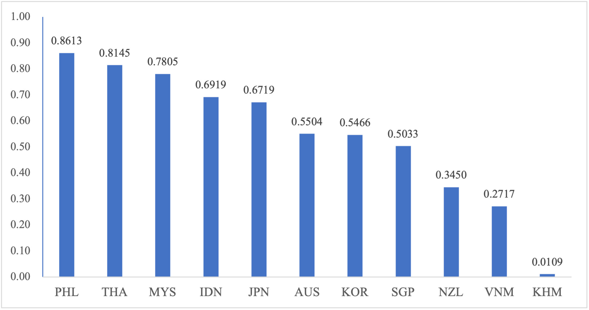
Export trade efficiency is the ratio of actual export value to export potential. Trade efficiency can be used to assess the development of China’s seafood exports to RCEP member countries (Figure 1).

Figure 1.Average Trade Efficiency of China’s Aquatic Product Exports to RCEP Member Countries

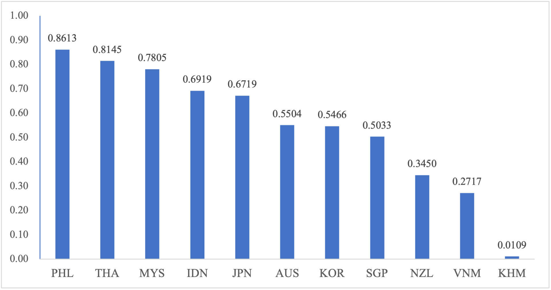
According to the formula for calculating trade efficiency mentioned earlier, the average trade efficiency of China’s aquatic products trade with RCEP member countries during the sample year was approximately 0.55. The chart above presents the average trade efficiency of China’s aquatic products exports to RCEP member countries. It can be observed that export trade efficiency varies significantly across different countries. The three countries with the highest trade efficiency are the Philippines, Thailand, and Malaysia, while New Zealand, Vietnam, and Cambodia exhibit the lowest trade efficiency.

When estimating trade efficiency using the Stochastic Frontier Gravity Model, high trade efficiency indicates fewer artificial restrictions and trade frictions between China and its trading partners; conversely, low efficiency suggests greater trade frictions. It is widely recognized that Japan and South Korea constitute China’s two primary seafood export markets, collectively accounting for approximately 50% of total exports. However, trade efficiency levels reveal that the efficiency of trade with these two countries does not correspond to their respective market shares. This indicates that while China exports significant volumes of seafood to Japan and South Korea, it simultaneously faces substantial artificial restrictions and barriers. To a certain extent, this suggests that substantial untapped trade potential remains between China and these nations.

5. Analysis of Factors Affecting Trade Inefficiencies

5.1. Estimation Results of the Stochastic Frontier Gravity Model under the “One-Step Method”

The likelihood ratio test has demonstrated the existence of trade inefficiency. This paper employs a one-step method to estimate the trade inefficiency model. To verify the stability of the model and regression results, both the trade facilitation value measured by principal component analysis and the trade facilitation calculated using simple arithmetic averaging were utilized, with results presented in Table 6. The overall model estimation is satisfactory. The λ value reported by the model represents the ratio of the standard deviation of the trade inefficiency term to the standard deviation of the random error term. The significant value of λ greater than 1 confirms that systematic and significant trade inefficiency factors indeed exist in the trade process, preventing trade from reaching its theoretical maximum.

The results from Table 8’s trade inefficiency model indicate that tariff levels exert a significant positive impact on trade inefficiency. This demonstrates that tariffs significantly impede China’s aquatic products trade, with higher tariff levels being more detrimental to exports—consistent with theoretical expectations. Conversely, trade facilitation levels exert a significant negative impact on trade inefficiency. That is, enhancing trade facilitation reduces trade inefficiency, thereby improving trade efficiency. Comparing the relative impacts of the two factors on trade inefficiency, trade facilitation exerts a greater influence. In other words, compared to reducing tariffs, enhancing trade facilitation is more conducive to promoting the development of aquatic products trade.

5.2. Results of Stochastic Frontier Gravity Models Across Different Dimensions of Trade Facilitation

As indicated by the core explanatory variables, trade facilitation is primarily composed of four sub-indicators: infrastructure (T), customs environment (C), government regulations (R), and finance and e-commerce (F). The impact of each sub-indicator on export efficiency may vary significantly. Analyzing using the composite trade facilitation index masks the heterogeneous effects of these sub-indicators on export efficiency. To derive more practically relevant conclusions, this study further examines the impact of the four primary indicators of trade facilitation development on export trade efficiency. Infrastructure (T), Customs Environment (C), Government Regulations (R), and Finance and E-commerce (F) are incorporated into a Stochastic Frontier Gravity Model, represented as Models 1, 2, 3, and 4 respectively. The regression results are presented in Table 7.

In Model (1), infrastructure passed the significance test at the 5% level, indicating that infrastructure can significantly enhance the efficiency of aquatic product trade while also highlighting its crucial role in this sector. For instance, live and premium chilled products demand strict timeliness and are typically transported by air, whereas frozen goods, canned products, and dried goods prioritize cost efficiency, making sea freight the predominant mode of transport.

In Model (2), the customs environment passed the significance test at the 1% level. Simplifying customs procedures and formalities will significantly reduce import and export processing times, enhancing trade efficiency while lowering the trade burden on enterprises.

In Model (3), government regulations passed the significance test at the 1% level. Taking the normalization and transparency of policy formulation by the government of the trading partner country as an example, timely publication of newly introduced or revised trade-related policies would help enterprises identify suitable business opportunities and partners based on the latest policy information. This would reduce transaction time costs and negotiation costs, thereby enhancing trade efficiency.

In Model (4), finance and e-commerce passed the significance test at the 10% level. High-quality e-commerce effectively promotes trade efficiency. E-commerce development centered on internet technology and information communication enables enterprises to complete import and export procedures, such as customs declaration, entirely online. This not only streamlines customs clearance processes and enhances the operational efficiency of transit agencies but also ultimately boosts trade efficiency.

In summary, different dimensions of trade facilitation exert varying impacts on inefficiencies in seafood trade. Compared to infrastructure, finance, and e-commerce, customs environments and government regulations exert a more significant influence on the efficiency of seafood trade.

Aquatic products are the trade category most susceptible to tariffs, trade remedies, and technical barriers. For Chinese aquatic product exporters, tariffs and trade facilitation are the two primary factors contributing to inefficiencies in aquatic product trade.

6. Conclusions and Recommendations

6.1. Main Findings

This paper constructs an indicator system for trade facilitation levels and incorporates it into the factors influencing trade inefficiency. It examines the impact of the trade facilitation levels of RCEP member countries on the efficiency of China’s aquatic product exports. The specific conclusions are as follows:

First, the average trade facilitation score for RCEP member states stands at 0.6448, indicating a generally moderate level of trade facilitation. This suggests that the overall trade facilitation environment and terms of trade within the RCEP region still hold significant room for improvement.

Second, the non-time-varying stochastic frontier model suggests that among the factors influencing China’s seafood exports, China’s GDP has a suppressive effect, although it is not statistically significant; conversely, the GDP of trading partner countries demonstrates a significant promoting effect. Distance emerges as a significant factor suppressing trade; meanwhile, shared language and the trade complementarity index exert a significant promoting effect on seafood trade.

Third, the trade inefficiency model demonstrates that tariffs and trade facilitation exert significant effects on trade inefficiency, with trade facilitation having a greater impact than tariffs. Among the four primary indicators of trade facilitation, customs environment and government regulations exert a more pronounced and substantial influence on trade inefficiency in aquatic products compared to infrastructure and finance and e-commerce.

Fourth, in terms of trade efficiency, China’s average efficiency in exporting aquatic products to RCEP member countries is approximately 0.55. However, this also indicates significant trade barriers between China and RCEP members, particularly for major aquatic product consumers like Japan and South Korea. China must further strengthen economic and trade cooperation with trading partners, foster a favorable trade environment, eliminate mutual trade barriers, enhance trade efficiency, and fully tap the potential of Chinese seafood exports. This will enable China to expand its seafood export volume to RCEP member countries beyond current levels.

6.2. Policy Implications

The findings of this paper reveal that elevating the level of trade facilitation significantly boosts both the development and efficiency of the aquatic products trade between China and RCEP member states. Accordingly, this paper formulates the following policy recommendations, primarily focusing on initiatives to enhance trade facilitation.

Firstly, enhancing infrastructure connectivity between China and RCEP member countries. To promote trade facilitation, it is essential to comprehensively develop and upgrade a seamless multimodal transport infrastructure network connecting China and RCEP member states. This involves fostering cooperation on infrastructure and extending technical and financial support to countries with insufficient capacities, thereby enhancing logistics efficiency across the free trade area.

Secondly, improve the customs environment. The optimization of the customs environment in RCEP member states can greatly promote the efficiency of China’s exports. To this end, China should pursue enhanced customs cooperation and dialogue with other members to elevate customs management standards jointly. This is instrumental in increasing trade facilitation across the free trade area and, concurrently, driving the expansion of China’s exports to RCEP markets.

Thirdly, create a sound regulatory environment. Elevating the regulatory environment across RCEP member states is conducive to China’s export efficiency. While political structures vary, the assessment of a sound regulatory environment is premised on universal factors. These encompass an independent judiciary, efficient dispute resolution through government policies, transparency and stability in the implementation process, and the capacity of policies to keep pace with societal evolution.

Lastly, promote finance and e-commerce. In the financial sector, efforts should leverage institutions like the ADB and AIIB to enhance infrastructure financing, encourage financial institutions to innovate in agricultural trade products, and increase support for farmers and enterprises through credit and insurance. In the e-commerce sector, priorities include strengthening information networks, supporting and regulating cross-border e-commerce platforms, and boosting regional logistics efficiency to facilitate the flow of agricultural products.

Acknowledgements

This paper is supported by the Later Stage Funding Project of the National Social Science Fund of China, “Research on China’s Foreign Trade Patterns and Transformation/Upgrading from the Perspective of Value-Added Trade Network Relationships” (No. 18FJY022); and the Major Research Special Project of the National Social Science Fund of China (No. 22VHQ006).

Authors’ contributions

Conceptualization: Chunxiang Hou (Lead). Data curation: Chunxiang Hou (Lead). Formal Analysis: Chunxiang Hou (Lead). Writing – original draft: Chunxiang Hou (Lead). Methodology: Zefang Liao (Lead). Writing – review & editing: Zefang Liao (Lead).

Declaration of Interest statement

The authors declare that they have no known competing financial interests or personal relationship that could have appeared to influence the work reported in this paper.

Declaration of generative AI in scientific writing

This paper does not involve the use of generative AI in scientific writing.

Data availability

Data will be made available on request.