Feed conversion ratio of Litopenaeus vannamei farming in China: evidence from multi-province surveys (2016–2023)

1. Introduction

China is one of the world’s largest aquaculture producers, and the performance of its aquaculture sector is increasingly evaluated not only by output growth but also by resource efficiency and environmental sustainability.^1,2 In 2022, global aquaculture production surpassed capture fisheries for the first time, reaching 94.4 million tonnes, of which China contributed approximately 57%.¹ In this context, feed efficiency has become a central concern because feed typically represents the highest variable cost in shrimp farming and is a major source of nutrient discharge into surrounding waters.^2,3 The feed conversion ratio (FCR), defined as the amount of feed required to produce a unit of biomass gain,⁴ is therefore a key indicator of both economic performance and environmental pressure: a lower FCR implies more efficient feed use, lower production costs, and reduced feed waste.

China’s policy framework has shifted markedly toward greener and higher-quality aquaculture development. While the 13^th Five-Year Plan (2016–2020) primarily emphasized expanding aquaculture production and distant-water fisheries, the 14^th Five-Year Plan (2021–2025) places greater emphasis on optimizing the layout of green nearshore aquaculture, developing marine ranches, and promoting ecological and healthy farming practices (MARA, 2021). This orientation was further reinforced by the 2020 No. 1 Central Document on rural revitalization, which explicitly advocated “green and healthy aquaculture.” These developments make it especially important to understand the farm-level determinants of feed efficiency in commercial aquaculture.

Among cultured shrimp species, Litopenaeus vannamei (Pacific white shrimp) is the dominant farmed shrimp in China and one of the most economically important species in the country’s aquaculture industry.⁵ Because of its economic weight, even modest improvements in FCR may have meaningful implications for both farm profitability and environmental performance.^3,6 Yet as the literature review below documents, existing evidence on shrimp FCR is dominated by nutritional and experimental studies, while micro-level evidence on how farmer characteristics, management behavior, and production organization shape FCR under commercial conditions remains limited—particularly for multi-province samples from China.^7–9

Against this background, this study examines the farm-level determinants of FCR in L. vannamei farming in China using survey data from four major shrimp-producing provinces during 2016–2023 (222 farms, n = 382 farm-cycle observations), focusing on branded-feed adoption and technical-service access and their effects on FCR both in the pooled sample and across traditional versus industrialized farming modes.

The study makes three contributions: (i) it offers multi-province micro-evidence on shrimp FCR determinants in China, complementing the nutrition-focused literature; (ii) it proposes a complementarity-matching hypothesis—a modern input’s marginal value depends on whether it relieves the production regime’s binding constraint; and (iii) it informs differentiated extension policy, prioritizing branded-feed promotion in traditional regimes and technical-service delivery in industrialized regimes.

2. Feed Conversion Ratio: Measurement Approaches, Determinants, Species-Specific Evidence, and Research Gaps

2.1. Measurement of feed conversion efficiency in aquaculture

Feed conversion efficiency in aquaculture is most commonly assessed through the feed conversion ratio (FCR), which links feed input directly to biomass gain and serves as an operational indicator of production performance.^3,4 At the farm level, FCR is particularly informative because it reflects both biological growth and managerial effectiveness in feed use.

A parallel literature has developed broader sustainability indicators, such as the fish-in:fish-out (FIFO) ratio^10–12 and the economically weighted eFIFO.¹³ These measures capture the upstream ecological burden of feed ingredients and are conceptually distinct from—though complementary to—farm-level FCR, which focuses on on-farm utilization efficiency.^2,3

A third stream examines feed-related performance using farm or household survey data. Amankwah and Quagrainie¹⁴ combined a double-hurdle model with propensity score matching to study feed-technology adoption in Ghana, while Joffre et al.^15,16 emphasized the role of social–ecological systems and farmer decision-making in Southeast Asian aquaculture. These studies highlight that feed efficiency is shaped not only by biology but also by management decisions and technology adoption—a perspective central to the present study.

2.2. Determinants of FCR in aquaculture

The determinants of FCR are typically grouped into nutritional and farm-management factors.

On the nutritional side, feed composition is a primary driver. Studies on protein levels, fishmeal substitution, and feed additives consistently find that the relationship between feed composition and FCR is non-monotonic: excessively high protein or fishmeal content does not necessarily improve feed efficiency.^7,17,18 Feed additives and raw material composition likewise significantly affect FCR.^19,20

On the farm-management side, feeding level, feeding frequency, stocking density, and environmental conditions all shape FCR.^21–25 Recent work further links labor intensity, water-quality monitoring, and biosecurity to production efficiency in commercial aquaculture.^26,27 However, literature on this aspect is dominated by controlled experiments and single-factor feeding trials. While valuable for identifying biological mechanisms, such designs offer limited evidence on how farmer behavior, production organization, and managerial inputs shape FCR under commercial conditions, where input choices are endogenous and self-selection is pervasive.^28,29

2.3. Research on FCR in Litopenaeus vannamei

Research on feed conversion efficiency in L. vannamei has developed relatively recently, driven by the rapid expansion of intensive shrimp farming and rising feed costs.^3,10 Nutritional studies confirm that the feed-composition–FCR relationship is nonlinear: extremely low-fishmeal diets reduce growth and feed efficiency,³⁰ and higher-quality fishmeal yields lower FCR than lower-quality fishmeal³¹ —evidence directly relevant to the present study’s focus on branded feed, which embodies higher and more consistent ingredient quality. Recent work has also explored the genetic basis of feed efficiency, with Dai et al.⁸ reporting moderate heritability of feed-efficiency traits under low-fishmeal and low-protein diets.

Management factors—stocking density, feeding strategy, water conditions, and production intensity—have likewise been recognized as important.^15,24,25 Nevertheless, most studies on L. vannamei rely on laboratory trials or breeding evaluations, and commercial-farm evidence remains scarce, particularly multi-province survey data capturing heterogeneity in farmer characteristics, farming practices, and production organization.

2.4. Research Gap and Positioning of This Study

The literature reveals two gaps. First, the Chinese literature on feed conversion remains dominated by finfish studies and experimental nutrition research, with limited evidence on how managerial inputs—branded-feed adoption and technical-service access—translate into FCR outcomes under real commercial conditions. Second, within the shrimp literature, micro-level behavioral and organizational determinants of FCR have received little attention, and almost no studies examine heterogeneous effects across production regimes. Yet the coexistence of traditional and industrialized systems in Chinese shrimp aquaculture^15,32,33 implies that the marginal value of any modern input likely depends on whether it matches the binding constraint of the production regime—a possibility that has not been systematically tested.

This study addresses both gaps by combining multi-province farm-level survey data (2016–2023) with a rigorous identification strategy (PSM, subsample heterogeneity analysis, Rosenbaum bounds, and OLS interaction tests), thereby complementing the dominant experimental literature with economic-behavioral evidence and providing empirical support for a complementarity-matching framework of input effectiveness.

3. Conceptual Framework and Research Hypotheses

3.1. Conceptual Framework

This study draws on human capital theory,^34–36 technology adoption theory,^37–39 and the theory of constraints⁴⁰ to explain how farmer characteristics and production decisions shape feed-use efficiency in L. vannamei farming. At the farm level, the feed conversion ratio (FCR) is determined not only by feed formulation and shrimp biology, but also by the farmer’s capacity to acquire and process information, adopt appropriate technologies, and organize production efficiently.^6,15,26

Three channels are emphasized. First, farmer human capital—particularly education and farming experience—may improve the precision of feeding, water-quality management, and disease prevention, thereby reducing feed waste.^19,41,42 Second, input and technology choices—such as the use of branded feed and the receipt of technical services—may affect feed quality, management standardization, and access to professional guidance, which in turn influence feed-use efficiency.^9,41,43 Third, production organization and management intensity—farming mode, stocking density, farm scale, and farming cycle length—shape biomass growth, environmental conditions, feeding precision, and biological risk, thereby affecting FCR.^24,25,44

Crucially, these three channels are not independent. Drawing on the theory of constraints,⁴⁰ the marginal value of any single input depends on whether it relieves the binding constraint of the production regime. In traditional pond farming, where feed quality is often the most limiting factor, branded feed adoption is expected to yield large efficiency gains, while technical services may have weaker effects because the binding constraint lies elsewhere. In industrialized farming, where feed quality is already relatively standardized but operational complexity and disease risk are high, technical services focused on water quality and biosecurity are expected to yield greater gains. We refer to this logic as the complementarity-matching hypothesis, which motivates the heterogeneity analysis in Section 6.

Accordingly, this study conceptualizes FCR as a farm-management outcome jointly determined by farmer capability, input choice, and production organization, rather than as a purely biological indicator. Because some management choices may be jointly determined by unobserved farmer ability or farm conditions, the empirical analysis uses propensity score matching to mitigate self-selection bias for the two focal binary inputs (branded feed and technical services), and supplements it with Rosenbaum bounds to assess sensitivity to unobserved bias. Remaining identification concerns are discussed in Section 4.4.

3.2. Research Hypotheses

Based on the framework above, the study advances four core hypotheses that correspond directly to the empirical analysis in Section 6.

Core hypotheses — average effects:

H1. Branded-feed adoption reduces shrimp FCR on average.

H2. Receipt of technical services reduces shrimp FCR on average.

Core hypotheses — complementarity-matching:

H3 (Feed). The FCR-reducing effect of branded feed is significantly stronger in traditional pond farming than in industrialized farming, because feed quality is the binding constraint in the traditional regime.

H4 (Service). The FCR-reducing effect of technical services is significantly stronger in industrialized farming than in traditional pond farming, because operational complexity and disease risk are the binding constraints in the industrialized regime.

For farmer human capital and production organization, the study posits the following directional predictions, tested jointly in the OLS specifications:

A1. Education is negatively associated with FCR.

A2. Farming experience is negatively associated with FCR.

A3. Stocking density is significantly associated with FCR; the sign may be negative if most farms operate below the technical optimum, but may weaken or reverse at excessive densities.

A4. The industrialized farming mode is significantly associated with FCR relative to traditional pond farming, with direction ambiguous ex ante.

A5. A longer farming cycle is positively associated with FCR.

A6. Farming scale is significantly associated with FCR, with direction ambiguous due to competing effects of economies of scale and managerial complexity.

Gender, province, and survey year are included as controls without directional hypotheses. All hypotheses and corresponding variables are summarized in Section 4.3.

4. Data and Methods

4.1. Data source and sample

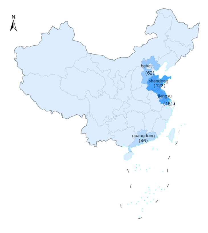
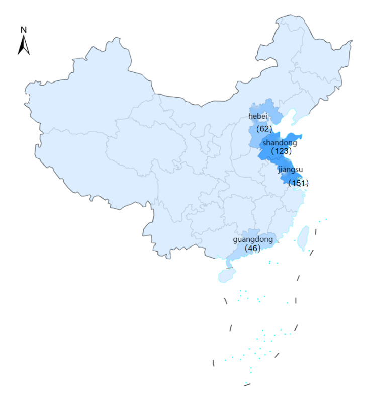
This study focuses on four major Litopenaeus vannamei-producing provinces in China—Shandong, Hebei, Jiangsu, and Guangdong—which span the principal aquaculture zones along the northern, eastern, and southern coasts and capture substantial heterogeneity in climate, farming systems, and management practices (Figure 1) Within these provinces, fieldwork concentrated on the leading shrimp-producing prefectures: Lianyungang (Jiangsu), Rizhao (Shandong), Zhanjiang (Guangdong), and Tangshan and Cangzhou (Hebei).

Figure 1.Geographic distribution of the survey areas

Data source: Field surveys conducted by authors’ team.
Base map source: Standard Map Service website of the Ministry of Natural Resources (http://bzdt.ch.mnr.gov.cn/index.html); map data from China Map Publishing House and the National Geomatics Center of China.

The data come from annual field surveys conducted by the authors’ team between 2017 and 2023. Because each survey wave collected production records covering the most recent completed grow-out cycle as well as recall data on earlier cycles, the resulting production records span the 2016–2023 farming seasons. Survey coverage in Hebei began only in 2019; the resulting dataset therefore constitutes an unbalanced pooled cross-section rather than a balanced panel (see Table 1).

Primary information was collected through face-to-face interviews with farmers and farm managers by trained investigators, with each interview lasting approximately 20–25 minutes. Respondents provided detailed production information on feed use, stocking, harvesting, farming practices, and farmer characteristics. The questionnaire instrument and a summary of the main data items are provided in Appendix A.

The original dataset contained 690 observations. To ensure accurate FCR calculation, the sample was restricted to observations corresponding to a single, complete grow-out cycle with clearly identifiable input and output boundaries. Observations were excluded if they: (i) involved mixed-species farming; (ii) relied primarily on natural rather than commercial formulated feed; (iii) contained overlapping multi-crop records that prevented clean attribution of feed input to a single batch; or (iv) lacked key variables required for FCR calculation. After cleaning, 382 valid farm-cycle observations from 222 unique farms remained, distributed across provinces as Jiangsu 151 (39.5%), Shandong 123 (32.2%), Hebei 62 (16.2%), and Guangdong 46 (12.0%). The annual distribution is reported in Table 1.

4.2. Outcome variable: FCR

The feed conversion ratio (FCR) is a standard indicator of feed-use efficiency in aquaculture.^3,4 Following Zhuang et al.,⁴⁵ farm-level FCR is defined as:

\[{FCR}_{i} = W_{pi}/\left( W_{2i} - W_{1i} \right) \tag{1}\]

where \(W_{pi}\) is total feed input (kg), and \(W_{1i}\) and \(W_{2i}\) are stocked and harvested biomass (kg), respectively. A lower FCR indicates higher feed-use efficiency. All quantities reported in jin were converted to kilograms (1 jin = 0.5 kg).

Feed input (\(W_{p}\)). Because commercial pellet feed accounts for the dominant share of feed use in L. vannamei farming, \(W_{p}\) is measured by pellet-feed consumption recorded in the survey (brand, unit price, purchased quantity, and total expenditure). The live feed is excluded from the baseline calculation, as its reported use is limited and not consistently measured across farms.

Harvested biomass (\(W_{2}\)). \(W_{2}\) is taken directly from the reported harvest output of the grow-out cycle.

Stocked biomass (\(W_{1}\)). \(W_{1}\) was not recorded directly in the questionnaire. Because shrimp seed typically passes through a nursery stage before pond stocking and actual stocking sizes vary across farms,¹⁸ this study adopts a standardized stocking weight of 0.38 g per juvenile (≈3 cm body length; Li et al., 2020):

\[\begin{matrix} W_{1i} = N_{i} \times 0.00038\text{~kg} & & \end{matrix} \tag{2}\]

where \(N_{i}\) is the number of stocked juveniles. This standardization may introduce measurement error if true stocking weights vary systematically across regions or production regimes; the implications for interpretation are discussed in Section 7.3, and future surveys should record farm-specific stocking weights.

4.3. Explanatory Variables

The dependent variable is the farm-level FCR (Section 4.2). Explanatory variables follow the four categories summarized in Table 2 : farmer human capital (Gender, Education, Experience), input and technology adoption (Brand, Tech Service), production organization and management (Mode, Scale, Density, Cycle), and locational/temporal controls (province and year dummies). Brand and Tech Service serve as the two focal treatment variables: Brand corresponds to H1 (and H3), and Tech Service to H2 (and H4) (Table 2). The underlying mechanisms have been developed in Section 3 and are not restated here.

4.4. Empirical Strategy

The empirical analysis proceeds in three stages, designed to move from descriptive associations to the identification of core treatment effects and, finally, to a test of the complementarity-matching hypothesis.

4.4.1. Three-stage estimation strategy

Stage 1: Baseline OLS regression. The baseline specification is a pooled cross-sectional OLS regression of FCR on all explanatory variables, with province and year fixed effects:

\[\begin{aligned} FCR_{i} &= \alpha + \beta_{1}\text{Brand}_{i} + \beta_{2}\text{TecService}_{i}\\ & \quad + X_{i}^{\prime}\gamma + \mu_{p} + \tau_{t} + \varepsilon_{i} \end{aligned}\tag{3}\]

where \(X_{i}\) collects farmer human-capital and production-organization controls, \(\mu_{p}\) and \(\tau_{t}\) denote province and year fixed effects, and standard errors are clustered at the farm level. Stage 1 provides conditional correlations and serves as a benchmark for the matched estimates in Stage 2.

Stage 2: Propensity score matching. To mitigate self-selection bias in the two focal binary treatments, we estimate the average treatment effect on the treated (ATT) of Brand and Tech Service via propensity score matching. For each treatment, a logit model regresses the treatment indicator on the full set of covariates in Equation (3) (excluding the other focal treatment to avoid bad controls), generating estimated propensity scores. The baseline matching estimator is nearest-neighbor matching with replacement (k = 1), with kernel matching reported as a robustness check. Common-support and covariate-balance diagnostics are presented in Section 6.3. Sensitivity to hidden bias is assessed via Rosenbaum bounds, reporting the critical Γ at which the significance of the ATT would be overturned.

PSM is applied separately to (i) the pooled sample, (ii) the traditional-pond subsample, and (iii) the industrialized subsample. The contrast between (ii) and (iii) provides the primary test of the complementarity-matching hypothesis (H3, H4).

Stage 3: OLS interaction tests. As an independent check on the subsample PSM evidence, Equation (3) is augmented with interaction terms between each focal treatment and the industrialized-mode dummy:

\[\begin{aligned} FCR_{i} &= \alpha + \beta_{1}\text{Brand}_{i} + \beta_{2}\text{TecService}_{i}\\ & \quad + \beta_{3}\text{Mode}_{i} + \delta_{1}(\text{Brand}_{i} \times \text{Mode}_{i})\\ & \quad + \delta_{2}(\text{TecService}_{i} \times \text{Mode}_{i})\\ & \quad + X_{i}^{\prime}\gamma + \mu_{p} + \tau_{t} + \varepsilon_{i} \end{aligned}\tag{4}\]

Under H3, \(\delta_{1} > 0\) (the FCR-reducing effect of branded feed is weaker in industrialized farming). Under H4, \(\delta_{2} < 0\) (the FCR-reducing effect of technical services is stronger in industrialized farming). Significant \(\delta_{1},\delta_{2}\) with the predicted signs, replicating the subsample PSM pattern, would jointly support the complementarity-matching framework.

4.4.2. Endogeneity, identification, and interpretation

Three identification concerns merit explicit discussion.

(1) Selection on unobservables. PSM addresses self-selection on observed covariates but cannot eliminate bias from unobserved time-varying factors—for example, an unobserved dimension of farmer ability that drives both branded-feed adoption and careful feeding practices. Rosenbaum bounds quantify the magnitude of hidden bias required to overturn the ATT estimates (Section 6.3.6).

(2) Reverse causality. Because Brand and Tech Service are decisions made at or before stocking, while FCR is realized only at harvest, reverse causality from FCR to treatment status within the same cycle is structurally unlikely. Persistent reverse causality across cycles (farmers with chronically high FCR seeking out branded feed or services) would bias estimates toward zero and therefore work against finding the observed FCR-reducing effects.

(3) Measurement error. Stocked biomass is computed using a standardized juvenile weight (Section 4.2); systematic regional or regime-specific deviations from 0.38 g would affect FCR levels but not, under plausible assumptions, the sign of treatment-effect heterogeneity across regimes. The implications and possible refinements are discussed in Section 7.3.

Taken together, the three-stage strategy—OLS, PSM with subsample heterogeneity, and OLS interaction tests, all subject to Rosenbaum sensitivity analysis—provides converging evidence on the average effects (H1, H2) and on the complementarity-matching mechanism (H3, H4) examined in Section 6.

5. Descriptive Statistics

5.1. Overview of FCR Changes

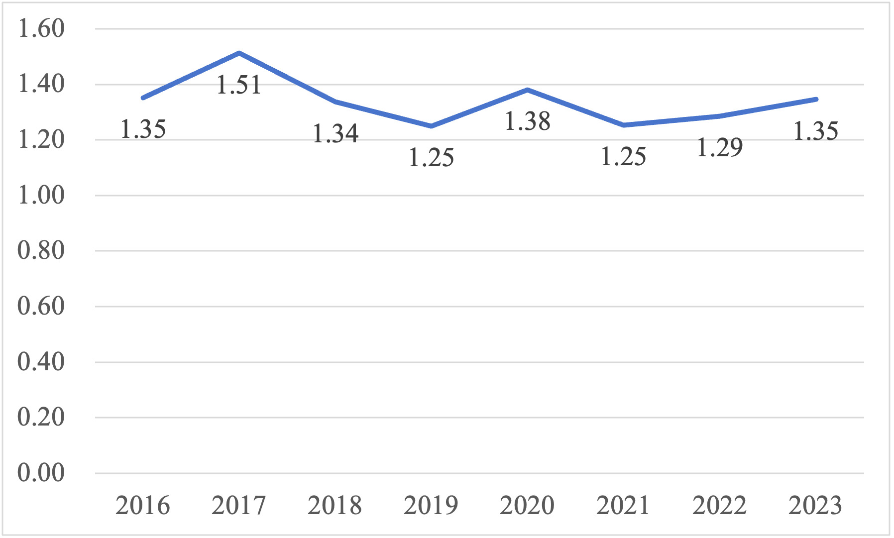
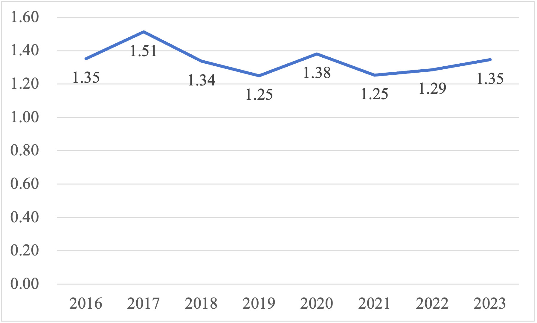
Between 2016 and 2023, the annual mean FCR of Litopenaeus vannamei farming in the sampled provinces fluctuated between 1.25 and 1.51, without exhibiting a clear monotonic trend (Figure 2). The highest annual mean was recorded in 2017 (1.51), while the lowest values occurred in 2019 and 2021 (both 1.25). The temporary increase in 2020 (1.38) coincided with COVID-19-related disruptions to input supply and on-farm management,⁴⁶ after which the mean returned to its earlier low in 2021. From 2022 to 2023, annual means rose modestly from 1.29 to 1.35. The pooled mean FCR across all 382 farm-year observations is 1.322. Comparing the starting and ending years suggests that average feed-use efficiency has remained broadly stable rather than improved over the sample period, while substantial within-year heterogeneity persists.

Figure 2.Annual mean FCR of Litopenaeus vannamei, 2016–2023.

Source: Compiled by the authors based on field surveys.

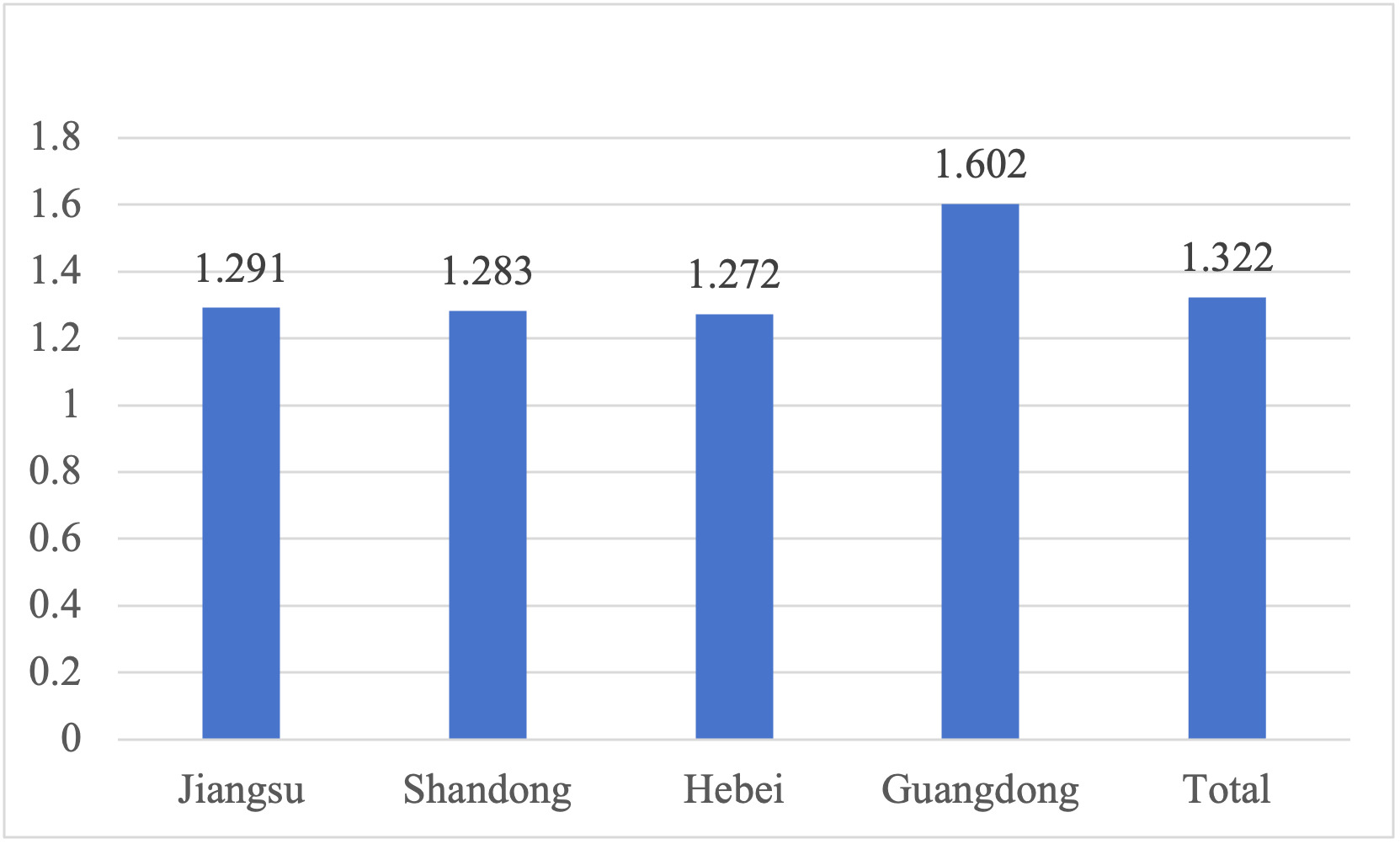
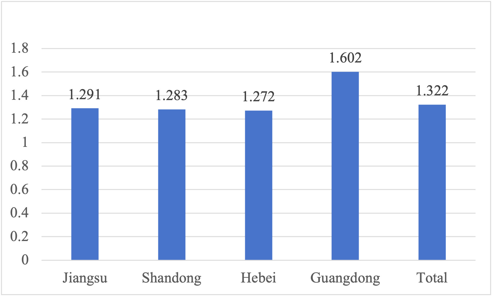
Substantial regional heterogeneity is also observed (Figure 3). Jiangsu (1.291), Shandong (1.283), and Hebei (1.272) all report mean FCR values below the overall sample average of 1.322, indicating relatively higher feed-use efficiency. In contrast, Guangdong reports a mean FCR of 1.602—approximately 0.28 above the overall sample average and roughly 0.30 higher than each of the other three sampled provinces. Because higher FCR values correspond to greater feed consumption per unit of harvested biomass, these results indicate a noticeable feed-use efficiency gap between Guangdong and the three northern/eastern provinces. This regional contrast may reflect differences in farming-mode composition, water temperature, disease pressure, and management intensity—patterns examined in the multivariate analysis (Section 6) and motivating the use of province fixed effects with Shandong as the reference category.

Figure 3.Mean FCR of Litopenaeus vannamei by province, 2016–2023.

Source: Compiled by the authors based on field surveys.

5.2. Farmer and farming characteristics

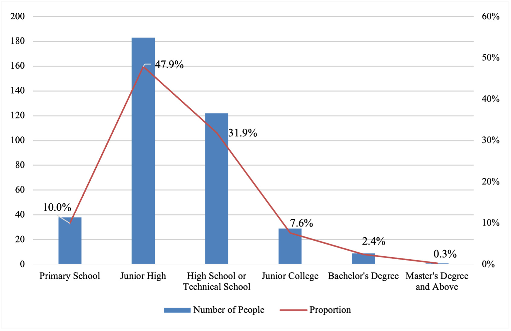
This subsection summarizes the sample’s farmer and farm characteristics, with descriptive patterns of the focal variables presented in Figures 4- 8.

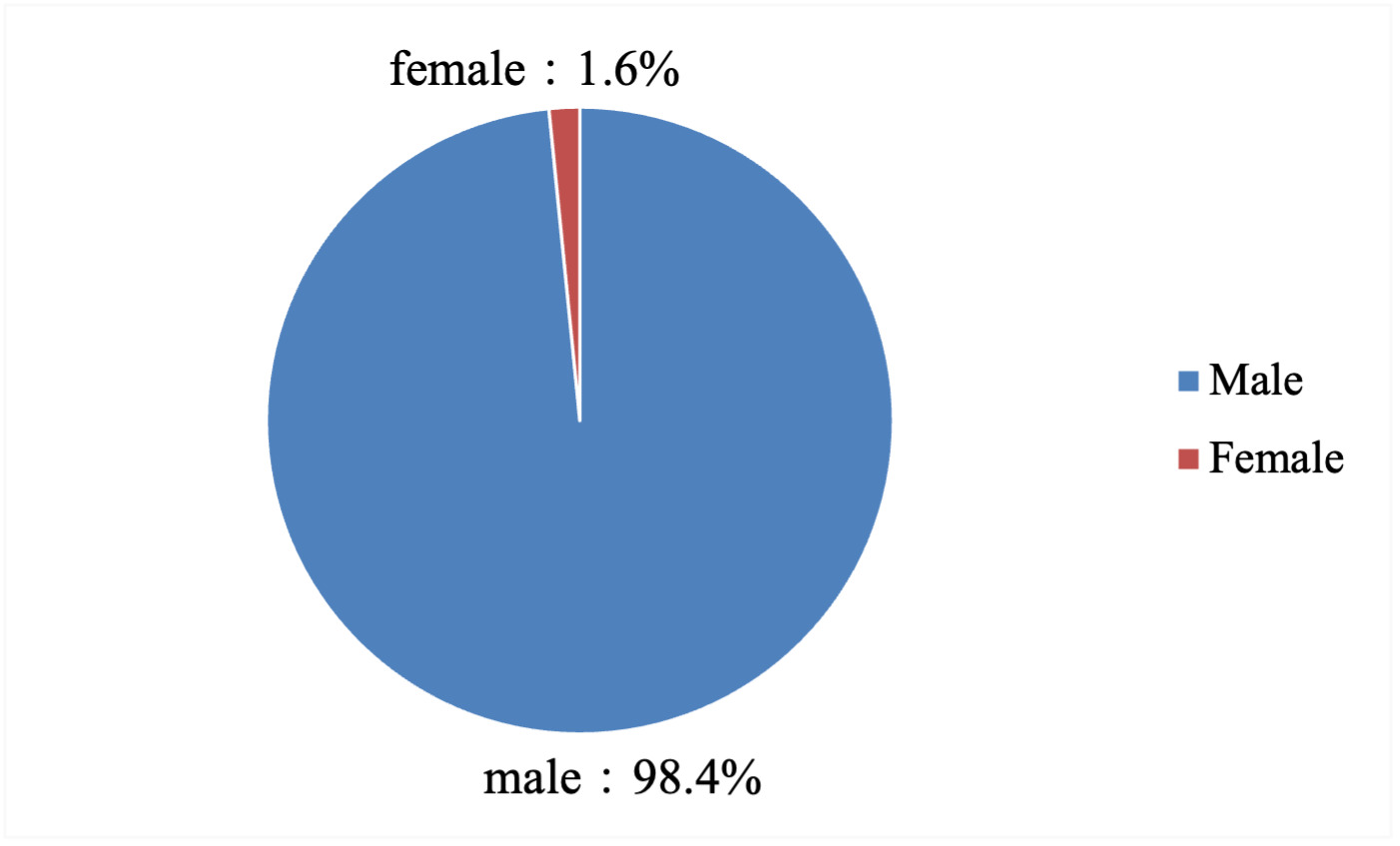
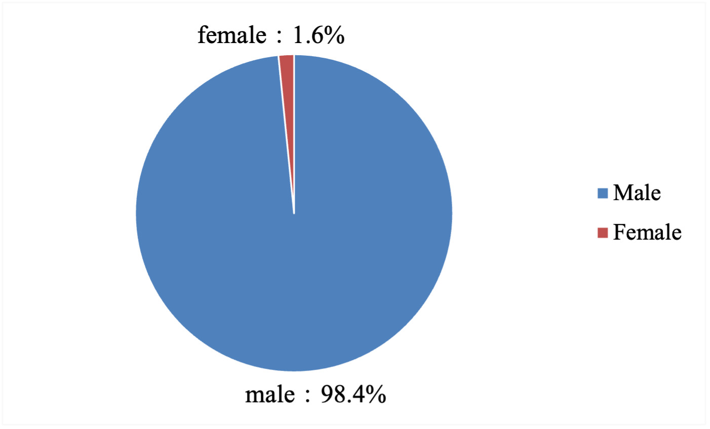
Gender. Male farmers account for the overwhelming majority of respondents. Among the 382 valid observations, 376 (98.43%) are male, and 6 (1.57%) are female (Figure 4). This distribution is broadly consistent with the gender composition of the on-site management workforce in Chinese shrimp farming, where male farmers traditionally take primary responsibility for pond operations. Given the strong imbalance, gender is included as a control rather than a focal variable.

Figure 4.Gender composition of surveyed farmers

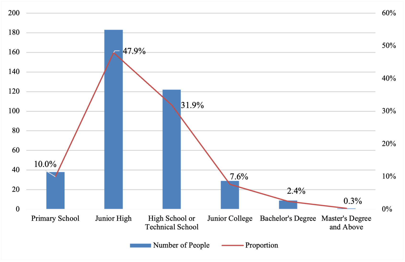
Education. Educational attainment is concentrated at the junior-high and senior-high / technical-secondary levels. Following the classification of the National Bureau of Statistics, respondents are grouped into six categories (Figure 5): 38 (9.95%) completed primary school, 183 (47.91%) junior high, 122 (31.94%) senior high or technical secondary, 29 (7.59%) hold a junior college diploma, 9 (2.36%) a bachelor’s degree, and 1 (0.26%) a master’s degree or above. Overall, about 90% of respondents completed at most senior high or technical-secondary school, indicating that formal higher education remains relatively uncommon among shrimp farmers in the sample. This profile is consistent with the broader pattern documented for Chinese aquaculture households.⁴²

Figure 5.Educational attainment of shrimp farmers

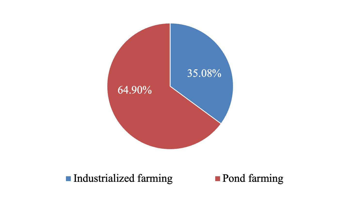
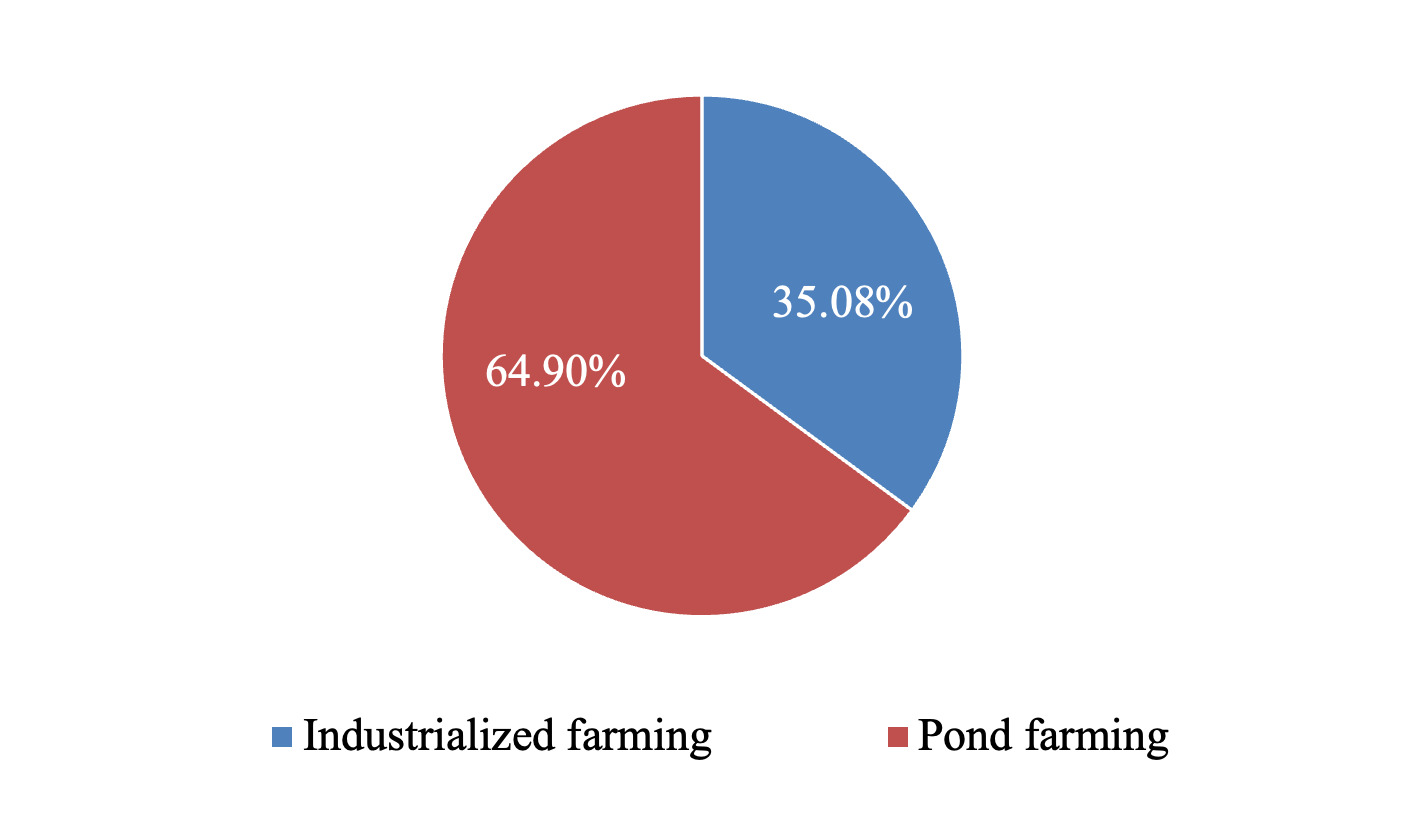
Farming mode. Farming modes are classified as industrialized or traditional pond farming. Among the 382 respondents, 134 (35.08%) operate under the industrialized mode and 248 (64.92%) under the traditional pond mode (Figure 6). Traditional pond farming, therefore, remains the dominant production model. The roughly 35:65 split provides sufficient variation for the subsample heterogeneity analysis in Section 6.3, which tests the complementarity-matching hypotheses H3 and H4.

Figure 6.Distribution of farming modes

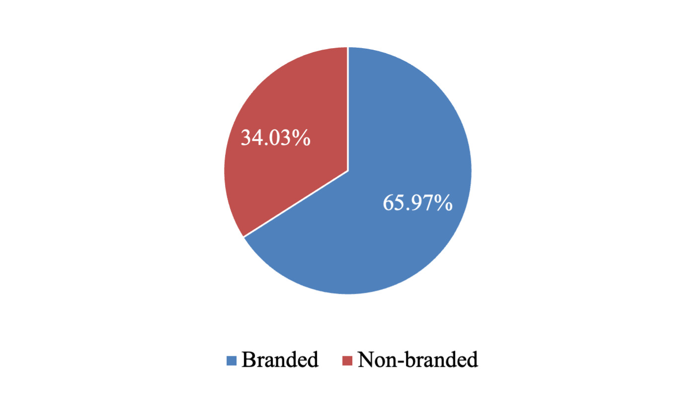
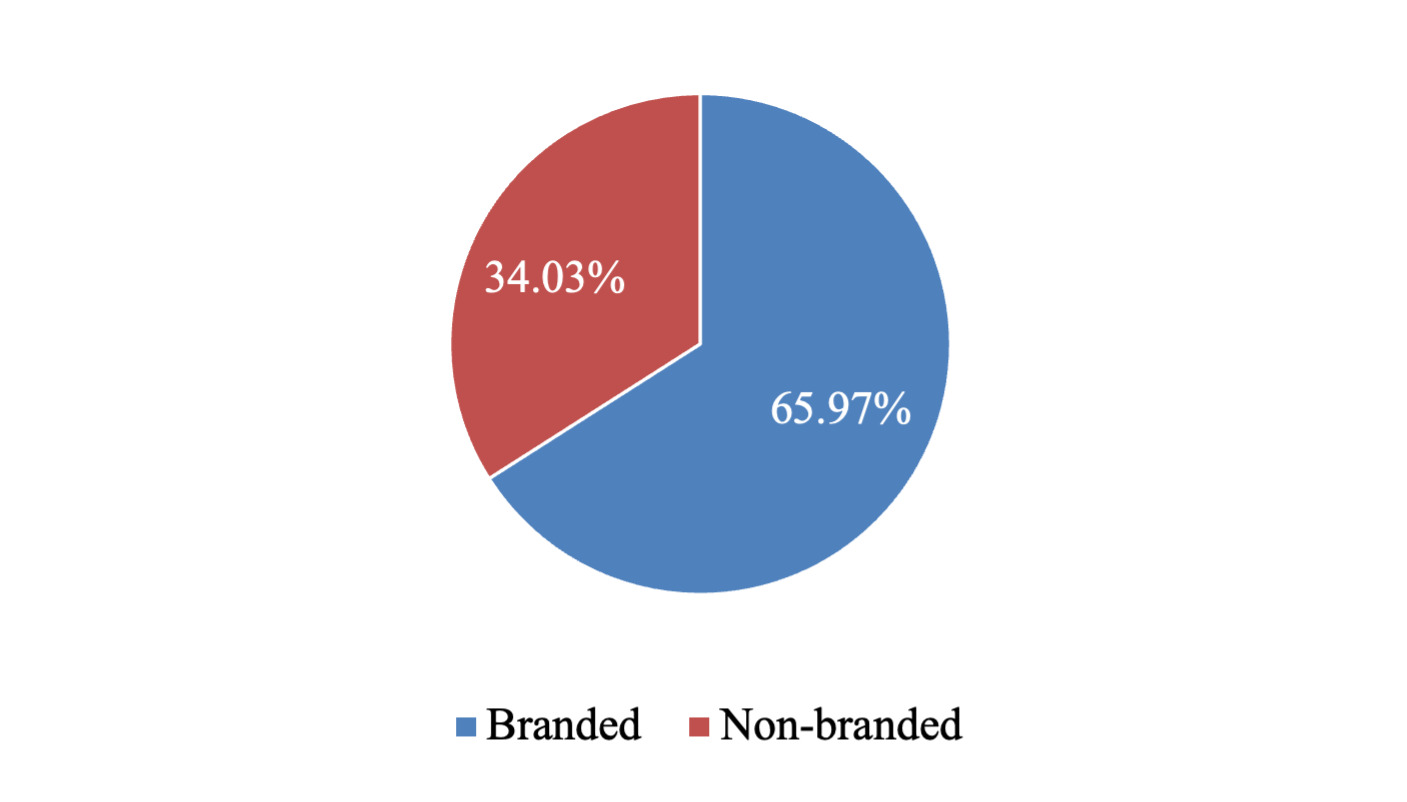
Feed brand. Feed inputs are classified as branded or non-branded (Figure 7): 252 respondents (65.97%) primarily use branded commercial pellet feed produced by formal manufacturers, while 130 (34.03%) primarily use non-branded feed sourced from small-scale local mills or self-prepared mixes. The roughly 66:34 split ensures adequate treatment-control variation for the PSM analysis of Brand in Section 6.2.

Figure 7.Selection of feed brands by farmers

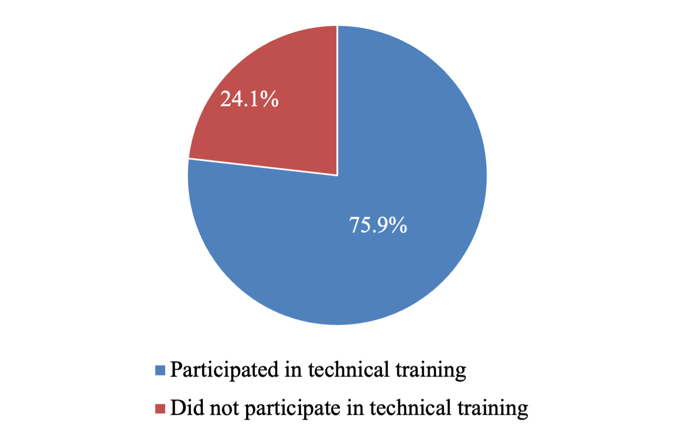
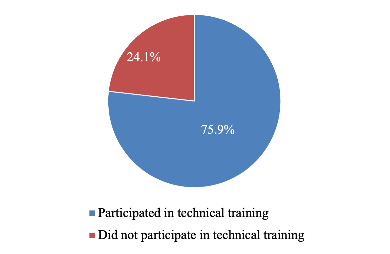
Technical services. Respondents are classified by whether they received technical training during the production cycle. Among the 382 respondents, 290 (75.92%) reported having received training, while 92 (24.08%) had not (Figure 8). Field interviews indicate that technical services are typically delivered through four channels: extension activities organized by local agricultural technology stations, on-site training provided by leading feed and aquaculture enterprises, training organized by industry associations, and online support delivered through digital information platforms. The dominance of public extension and enterprise-led training reflects the dual-track structure of agricultural technology delivery in China.⁴⁷ The non-trivial untreated share (24%) provides a valid comparison group for the PSM analysis of Tech Service in Section 6.2.

Figure 8.Farmer participation in technical service programs

5.3. Bivariate FCR Comparisons by Treatment Status

Table 3 reports unconditional mean FCR comparisons across the two focal binary treatments and the production-regime dimension. These bivariate patterns preview the core hypotheses but should be interpreted with caution, as they do not control for confounding factors.

Three patterns are noteworthy. First, in the full sample (Panel A), both Brand and Tech Service are associated with significantly lower FCR—by 0.185 (p = 0.003) and 0.205 (p = 0.003) feed units per kilogram of harvested shrimp, respectively—providing preliminary support for H1 and H2. Second, the Brand effect is statistically significant in traditional pond farming (Δ = 0.200, p = 0.007) but not in industrialized farming (Δ = 0.152, p = 0.195), consistent with the complementarity-matching prediction of H3: when feed quality is the binding constraint, as in traditional ponds, branded feed delivers larger efficiency gains. Third, the pattern is sharply reversed for Tech Service: the effect is only marginally significant in traditional farms (Δ = 0.140, p = 0.073) but more than three times larger and highly significant in industrialized farms (Δ = 0.465, p = 0.003), supporting H4. Because operational complexity, water-quality management, and disease pressure rise sharply in intensive systems, technical services that address these binding constraints produce disproportionately large efficiency gains. These bivariate patterns are suggestive but not causal; the multivariate OLS analysis in Section 6.1 and the PSM analyses in Section 6.2 formally test these hypotheses while controlling for confounders.

6. Empirical Results

6.1. Baseline OLS Results

Table 4 reports the baseline OLS estimates of Equation (3) under five progressively richer specifications. Column (1) includes only farmer demographics; Column (2) adds farm-management variables; Column (3) introduces the three focal policy-relevant variables (Brand, Tech Service, Mode); Column (4) adds province fixed effects; and Column (5), the preferred specification, further adds year fixed effects and clusters standard errors at the province × year level (29 clusters) to allow for arbitrary correlation among farms operating in the same provincial market in the same year.

6.1.1. Focal variables: Brand, Tech Service, and Mode

The adoption of branded feed is associated with a reduction in FCR of 0.159 units (p = 0.051) in the preferred specification, and the coefficient is remarkably stable across columns (3) – (5), ranging from −0.143 to −0.159. The receipt of technical services is associated with an even larger FCR reduction of 0.203 units (p = 0.035), also stable across specifications. These results provide preliminary support for H1 and H2, although a causal interpretation requires the PSM analysis in Section 6.2.

The coefficient on Mode displays a striking sign reversal between Column (3) and Columns (4) – (5): without province fixed effects, industrialized farming appears (insignificantly) associated with lower FCR; once provincial heterogeneity is absorbed, industrialized farming is associated with FCR that is 0.631 units higher (p = 0.001) than traditional pond farming. This pattern reflects classic Simpson-type confounding: Guangdong has both the highest share of industrialized farms and the highest mean FCR (Figure 3), so failing to control for province fixed effects masks the within-province effect of farming mode. The positive within-province coefficient is consistent with industrialized farms operating at higher biomass densities and facing greater biosecurity challenges, which raise feed requirements per unit of output. This average effect, however, masks substantial heterogeneity across the Brand × Mode and Tech Service × Mode margins, which is the focus of Section 6.3.

6.1.2. Human Capital and Farm-Management Controls

Among auxiliary predictions, the evidence is mixed but largely consistent with prior expectations:

Education (A1): strongly negative (−0.122, p < 0.001) — supports A1. Each additional level of formal schooling is associated with a 0.12-unit reduction in FCR.

Experience (A2): significant and negative (−0.019, p = 0.005) — supports A2, consistent with learning-by-doing.

Ln (Density) (A3): strongly negative (−0.323, p < 0.001) — supports the under-optimal density interpretation of A3. Within the observed range, higher stocking density is associated with lower FCR, suggesting that most sampled farms operate below the technical optimum.

Cycle (A5): insignificant in the preferred specification — no support for A5 once province and year effects are controlled.

Ln (Scale) (A6): negative but only marginally significant in Column (4) and insignificant in Column (5) — ambiguous evidence on scale economies, consistent with the competing-effects argument in Section 3.2.

Age: negative and significant throughout, suggesting that older farmers achieve modestly better feed-use efficiency, possibly reflecting accumulated tacit knowledge beyond formal experience.

Gender: insignificant, consistent with the highly imbalanced gender distribution (98.4% male) reported in Section 5.2.

6.1.3. Fixed Effects and Model Fit

Adding province fixed effects (Column 4) raises R² sharply from 0.122 to 0.242, indicating that regional heterogeneity—particularly the Guangdong gap—accounts for a substantial share of FCR variation. Adding year fixed effects (Column 5) yields a modest additional improvement to R² = 0.248, consistent with the absence of a strong temporal trend documented in Figure 2. Estimated province fixed effects (not reported in Table 4; available on request) indicate that Guangdong exhibits a within-sample FCR premium of approximately +1.04 units relative to Shandong even after controlling for all observable farm characteristics, suggesting that unobserved environmental factors (water temperature, salinity, disease pressure) likely play an important role in the Guangdong–North China efficiency gap—a finding that warrants further investigation in future research.

6.1.4. Endogeneity Concerns and Identification Strategy

The OLS estimates in Section 6.1 should be interpreted with caution due to potential endogeneity arising from self-selection into branding and technical-service adoption. Farmers who adopt branded feed or seek technical training may systematically differ from non-adopters in unobservable dimensions such as managerial ability, risk preference, or access to credit, which simultaneously affect FCR. This generates a non-zero correlation between the treatment variable and the error term, biasing OLS estimates.

To address this concern, we employ Propensity Score Matching (PSM) following Rosenbaum and Rubin,⁴⁸ which constructs a counterfactual by matching treated farmers with observationally similar untreated farmers on a rich set of covariates. PSM relaxes the linearity assumption of OLS and explicitly addresses selection on observables. We further conduct Rosenbaum-bounds sensitivity analysis to assess robustness against selection on unobservables.

Formally, we estimate the Average Treatment Effect on the Treated (ATT):

\[\begin{aligned} \text{ATT} &= E\left\lbrack \text{ }Y_{i}(1) - Y_{i}(0)\text{ }|\text{ }D_{i} = 1\text{ } \right\rbrack\\ & = E\left\{ \begin{array}{l} E\lbrack\text{ }Y_{i} \mid D_{i} = 1,\text{ }p(X_{i})\text{ }\rbrack \\ \quad - E\lbrack\text{ }Y_{i} \mid D_{i} = 0,\text{ }p(X_{i})\text{ }\rbrack\text{ }|\text{ }D_{i} = 1 \end{array} \right\} \end{aligned}\]

where \(D_{i} \in \{ 0,1\}\) denotes treatment status, \(Y_{i}(1)\) and \(Y_{i}(0)\) are the potential outcomes (FCR) under treatment and control, and \(p(X_{i}) = \Pr(D_{i} = 1 \mid X_{i})\) is the propensity score estimated via logit.

6.2. PSM Results (Full Sample)

This section reports the PSM estimates for two treatment variables—branding adoption (Brand) and technical-service adoption (Tech Service)—using the full sample of 382 shrimp farmers. We proceed in three steps: (i) estimating the propensity score via logit; (ii) verifying covariate balance and common support; and (iii) computing the ATT under multiple matching algorithms to ensure robustness.

6.2.1. Propensity Score Estimation

We estimate the propensity score \(p(X_{i})\) separately for each treatment using a logit model that includes farmer demographics (age, gender, education), production characteristics (experience, farm size, cycle length, density), and year fixed effects.

The two selection equations reveal distinct mechanisms of adoption. Branding adoption is driven primarily by farmer age (β = 0.040, p < 0.05) and stocking density (β = 0.645, p < 0.01), suggesting that older farmers operating denser facilities are more likely to participate in branded supply chains—possibly reflecting accumulated reputational capital and stronger incentives to differentiate output through certified channels. Technical-service adoption is significantly associated with education (β = 0.491, p < 0.01) and marginally with density (β = 0.421, p < 0.10), consistent with the view that more educated farmers possess greater absorptive capacity to internalize external technical knowledge, while denser operations face stronger biosecurity pressures that incentivize professional consulting. The moderate Pseudo R² values (0.122 and 0.191) indicate that observables explain selection meaningfully but leave substantial overlap between treated and control groups—a desirable property for matching. Notably, the cross-treatment controls (Brand in column 2; Tech Service in column 1) are statistically insignificant, suggesting that the two adoption decisions are made largely independently conditional on farmer characteristics (Table 5).

6.2.2. Balance Tests and Common Support

A credible PSM estimate requires that matching eliminates systematic differences in observable covariates between treated and control units.⁴⁹ Table 6 reports the standardized percentage bias for each covariate before and after nearest-neighbor (1:1) matching, together with Rubin’s overall balance diagnostics.

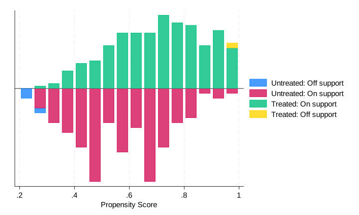
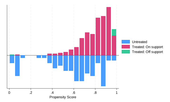
Interpretation. The balance diagnostics confirm that matching is highly effective for both treatments. Before matching, several covariates exhibit substantial imbalance—most notably ln(Scale) and ln(Density), with absolute biases exceeding 25%—and joint balance tests strongly reject equality of distributions (p < 0.01). After 1:1 nearest-neighbor matching, mean absolute bias falls to 7.0% in both samples, well below the conventional 10% threshold (Rosenbaum & Rubin, 1985). Rubin’s B drops from 49.6 to 23.5 (Brand) and from 80.5 to 24.1 (Tech Service), both meeting the B < 25 criterion. The joint balance tests are no longer rejected after matching (p = 0.546 for Brand; p = 0.417 for Tech Service), and the Pseudo R² collapses to 0.01 in both cases, suggesting substantial improvement in covariate balance (Table 6).

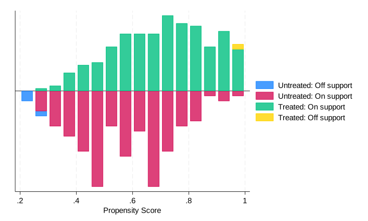
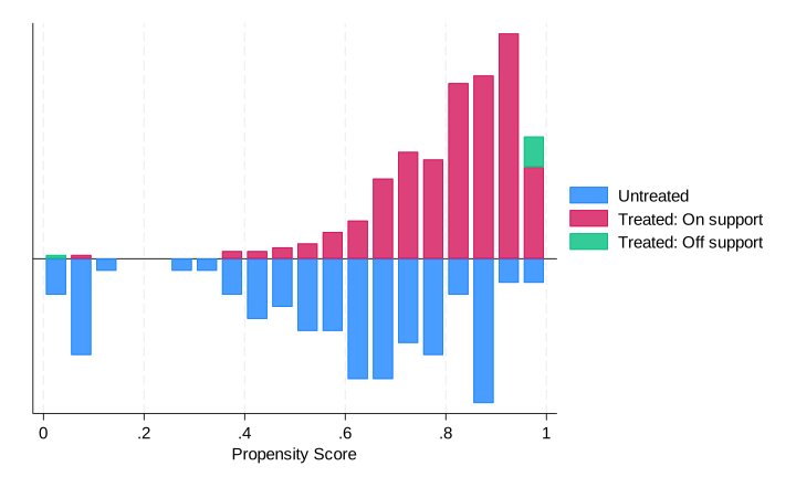
The common support condition is also reasonably satisfied. For the Brand treatment, 5 of 382 observations (1.3%) fall outside the common support region, leaving 377 observations for ATT estimation. For the Tec Service treatment, 9 observations (2.4%) are outside support, all from the treated group, leaving 373 matched units. Overall, the small number of off-support observations suggests substantial overlap in the propensity score distributions of treated and control units, supporting the validity of the matching procedure (Table 6).

Figure 9 and Figure 10 plot the kernel density of the estimated propensity scores before and after matching for each treatment, visually confirming that the post-matching distributions of treated and control units are nearly indistinguishable.

Figure 9.Propensity score distributions before and after matching (Brand treatment)

Figure 10.Propensity score distributions before and after matching (Tech Service treatment)

6.2.3. ATT Estimates

Having established that matching successfully balances observables and that common support holds, we now estimate the ATT of branding and technical-service adoption on FCR. To assess robustness to the choice of matching algorithm, we report three estimators: (i) nearest-neighbor matching (NN1) with one-to-one replacement; (ii) kernel matching using the Epanechnikov kernel with bandwidth 0.06; and (iii) radius matching with caliper 0.05. Table 7 reports the ATT estimates.

6.2.4. Robustness Checks

Robustness across algorithms. Table 7 demonstrates that the ATT estimates are remarkably stable across all three matching algorithms. For the Brand treatment, ATT estimates range narrowly from −0.369 (Kernel) to −0.413 (NN1), with a mean of −0.384—a span of only 0.044 FCR units, or roughly 11% of the central estimate. All three estimates are significant at the 1% level, with t-statistics between −3.54 and −4.12. The Kernel and Radius estimators, which exploit information from multiple control units and therefore tend to be more efficient, yield nearly identical point estimates (−0.369 vs. −0.371) and smaller standard errors (0.090 vs. 0.117 for NN1), consistent with theoretical expectations.²⁹

For the Tech Service treatment, ATT estimates range from −0.262 (NN1) to −0.307 (Radius), with a mean of −0.292. The Kernel and Radius estimators deliver substantially stronger statistical evidence (t = −3.41 and −3.51, both significant at 1%) than NN1 (t = −2.03, significant at 5%), suggesting that the NN1 estimate is somewhat conservative due to its reliance on a single matched control per treated unit. The convergence of Kernel and Radius results (−0.305 vs. −0.307; difference < 0.002) provides particularly strong evidence that the Tech Service effect is not an artifact of matching specification.

Taken together, the cross-algorithm consistency satisfies the robustness criterion advocated by Caliendo and Kopeinig²⁹: if matching estimates were driven by idiosyncratic features of a single algorithm (e.g., a poorly matched outlier in NN1), the three estimators would diverge substantially. Their convergence within a narrow band—combined with the successful balance tests in Section 6.2.2—strengthens the causal interpretation of the estimated effects.

6.3. Heterogeneity Analysis: The Moderating Role of Production Mode

6.3.1. Empirical Strategy

The full-sample ATTs reported in Section 6.2.3 may mask heterogeneity across production environments. Farms in our sample operate under two distinct regimes: industrialized production, characterized by closed houses, automated feeding, and environmental controls; and traditional pond farming, relying on open or semi-open ponds with manual management. These regimes differ in process standardization, execution precision, and the marginal value of external quality discipline, making regime-specific effects a priori plausible. We therefore re-estimate the PSM procedure separately on each subsample, applying the same three matching algorithms, the same covariate vector, and the same logit specification as in the baseline.

6.3.2. Subsample ATT Estimates

Table 8 reports the heterogeneous ATT estimates by production mode. Two striking patterns emerge. First, branding effects concentrate almost entirely in traditional farming: among traditional farmers, branded feed is associated with an FCR reduction of 0.50–0.61—approximately 50% larger than the full-sample estimate and highly significant across all algorithms. Among industrialized farmers, the same treatment produces a point estimate indistinguishable from zero. Second, technical-service effects exhibit a mirror-image pattern: the intervention reduces FCR by 0.31–0.40 among industrialized farmers (significant at 5% or better) but only 0.14–0.23 among traditional farmers (statistically insignificant).

6.3.3. The Symmetric Reversal

The two patterns together constitute a symmetric reversal of intervention effectiveness across production regimes:

The diagonal cells capture essentially all of the FCR-improving effect documented in this chapter; the off-diagonal cells are economically and statistically null. The pooled ATTs reported earlier are thus weighted averages of two non-overlapping mechanisms operating in two distinct populations, not estimates of a homogeneous causal effect.

6.3.4. Mechanistic Interpretation

The reversal admits a coherent interpretation grounded in the complementarity–substitution structure between intervention type and production technology.

Branding in traditional farming. In traditional production, the binding constraint on FCR is executional rather than informational: open-pond environments and manual feeding make it difficult to enforce consistent input use. Branding contracts impose external monitoring, standardized protocols, and traceability requirements—they function as “soft industrialization” by embedding discipline contractually rather than physically. Once production is already physically standardized (as in industrialized farms), this contractual discipline becomes redundant, and the marginal effect collapses to zero.

Technical services in industrialized farming. Technical extension, by contrast, delivers fine-grained recommendations whose marginal value is bounded by the fidelity of implementation. Industrialized facilities, with automated climate control and mechanized feeding, translate advisory inputs into practice with minimal loss; traditional ponds filter the same advice through manual labor and approximate controls, attenuating the productivity payoff. The Tech Service ATT more than doubles when moving from traditional to industrialized farms.

The two interventions and the two regimes thus form a strict pairwise complementarity structure—branding pairs with traditional production, technical extension pairs with industrialized production—while mismatched combinations yield negligible returns.

6.3.5 Robustness Checks for Heterogeneous Effects

The symmetric reversal documented in Section 6.3.3 is the central empirical finding of this chapter. To ensure that this pattern is not an artifact of the PSM procedure or driven by unobserved confounding, we conduct two complementary robustness checks: (i) replicating the heterogeneity using a fully parametric OLS specification with interaction terms (R1), and (ii) assessing sensitivity to hidden bias via Rosenbaum bounds (R2).

R1. OLS Interaction Specification

PSM is a semi-parametric estimator that relaxes linearity assumptions and explicitly addresses selection on observables through matching. A natural robustness check is to verify whether the heterogeneous effects survive under a conventional parametric specification. We re-estimate the baseline OLS model (Equation 3) augmented with two-way interaction terms:

\[\begin{aligned} \text{FCR}_{i} &= \alpha + \beta_{1}\text{Brand}_{i} + \beta_{2}\text{TechService}_{i} + \beta_{3}\text{Mode}_{i}\\ & \quad + \gamma_{1}(\text{Brand}_{i} \times \text{Mode}_{i}) + \gamma_{2}(\text{TechService}_{i} \times \text{Mode}_{i})\\ & \quad + X_{i}^{\prime}\delta + \mu_{p} + \tau_{t} + \varepsilon_{i}, \end{aligned}\]

where \(\gamma_{1}\) and \(\gamma_{2}\) capture the differential effects of branding and technical services in industrialized versus traditional farms. If the symmetric reversal is genuine, we expect \(\gamma_{1} > 0\) (branding less effective in industrialized farms) and \(\gamma_{2} < 0\) (technical services more effective in industrialized farms).

Table 9 reports three specifications: Column (1) includes only the Brand × Mode interaction; Column (2) includes only the Tech Service × Mode interaction; Column (3) includes both interactions simultaneously. All specifications control for the full covariate set, province fixed effects, year fixed effects, and cluster standard errors at the province × year level.

Interpretation. The joint specification (Column 3) reveals asymmetric evidence for the two treatments. The Tech Service × Mode interaction is negative and highly significant (−0.333, p = 0.006), confirming that technical services reduce FCR by an additional 0.33 units in industrialized farms relative to traditional farms. This parametric estimate aligns with the PSM-based difference: the subsample ATTs imply a differential of (−0.372) − (−0.170) = −0.202, which is directionally consistent despite differences in estimation strategy.

In contrast, the Brand × Mode interaction is positive but statistically insignificant (+0.060, p = 0.645). The point estimate suggests that branding is 0.06 FCR units less effective in industrialized farms, consistent with the PSM finding that the Brand ATT is near zero in the industrialized subsample. However, the lack of statistical significance indicates that OLS—constrained by linearity and homoskedasticity assumptions—has insufficient power to detect this heterogeneity in the relatively small industrialized subsample (N = 134). The PSM estimator, by constructing a locally balanced comparison and allowing for non-linear propensity score effects, is better suited to uncover treatment-effect heterogeneity in small subsamples.⁵¹

Marginal effects: To facilitate comparison with the PSM ATTs, we compute treatment effects conditional on production mode from the joint specification:

The OLS and PSM estimates agree qualitatively on the direction and statistical significance of the Tech Service heterogeneity. For branding, OLS detects a marginally significant effect in traditional farms (p = 0.08) but underestimates the magnitude relative to PSM (−0.185 vs. −0.532), likely because OLS imposes a linear functional form that averages over non-linear selection patterns. The convergence of the two methods on the sign and significance pattern—despite their different identifying assumptions—strengthens confidence that the symmetric reversal is not a methodological artifact.

R2. Sensitivity to Hidden Bias: Rosenbaum Bounds

The PSM estimates rely on the conditional independence assumption (CIA): conditional on observed covariates, treatment assignment is as good as random. If unobserved factors simultaneously affect both treatment adoption and FCR, the ATT estimates may be biased. Rosenbaum bounds⁵² quantify how strong such hidden bias would need to be to overturn the conclusions.

The sensitivity parameter Γ represents the odds ratio of differential treatment assignment due to unobserved factors. Γ = 1 corresponds to the CIA (no hidden bias); Γ = 2 means that two observationally identical farmers could differ in their odds of treatment by a factor of 2 due to unobservables. For each subsample–treatment combination, we report the critical Γ at which the upper-bound p-value first exceeds 0.10, rendering the ATT statistically insignificant (Table 10).

All significant ATTs withstand Γ ≥ 2.8, well above the Γ > 2.0 benchmark for “strong robustness” in observational studies^52,53 (Table 10). Invalidating the core findings would require an unobserved confounder that nearly triples the odds of treatment adoption while being perfectly correlated with FCR—implausible given the richness of our covariate set.

Summary

Both checks support the symmetric reversal as a genuine feature of the data. OLS independently replicates the Tech Service heterogeneity at the 1% level and reproduces the qualitative pattern for branding; Rosenbaum bounds confirm that the PSM estimates are insensitive to plausible levels of hidden bias. The heterogeneous effects documented in Section 6.3.3 thus reflect true complementarities between intervention type and production technology rather than methodological artifacts.

7. Conclusions and Recommendations

7.1. Main Conclusions

Using farm-level survey data from 222 Litopenaeus vannamei farms across four major Chinese producing provinces over 2016–2023 (n = 382), this study identifies the effects of two managerial inputs—branded-feed adoption and technical-service access—on the feed conversion ratio (FCR), and tests whether their effectiveness depends on the production regime. Four conclusions emerge.

First, both managerial inputs improve feed-use efficiency on average. Pooled-sample PSM estimates indicate that branded feed and technical services each lower FCR by approximately 0.24–0.31 units, equivalent to a 15–20% reduction in feed waste per kilogram of shrimp harvested. The OLS baseline and unconditional mean comparisons corroborate these magnitudes, supporting H1 and H2.

Second, the average effects mask a sharp regime-dependent reversal. Among traditional pond farmers, branded feed substantially reduces FCR (ATT = −0.528, p < 0.01), whereas technical services have no significant effect. Among industrialized farmers, the pattern reverses entirely: technical services significantly reduce FCR (ATT = −0.376, p < 0.01) while branded feed has no detectable effect. This symmetric reversal—confirmed by OLS interaction tests (Tec × Mode = −0.333, p < 0.01) and robust to Rosenbaum bounds up to Γ ≈ 2.8–3.0—supports H3 and H4.

Third, the evidence validates a complementarity-matching mechanism. Consistent with the theory of constraints,⁴⁰ the marginal value of a modern input depends on whether it relieves the binding constraint of the prevailing production regime. In traditional ponds, where feed quality is the dominant bottleneck, branded feed delivers large efficiency gains; in industrialized systems, where feed quality is already standardized but operational complexity and biosecurity risks bind, technical services become the critical lever. Inputs deployed against non-binding constraints yield negligible returns.

Fourth, the findings extend the FCR literature from biology to behavior. While the existing literature on shrimp FCR is dominated by nutritional experiments and breeding trials, this study provides multi-province commercial-farm evidence that managerial inputs and production organization are first-order determinants of feed efficiency, and that their effectiveness cannot be assessed independently of the production context.

7.2. Policy Recommendations

The complementarity-matching framework implies that uniform extension policy is inefficient; targeted designs aligned with the binding constraint of each regime will yield substantially higher returns. Four recommendations follow.

(1) Differentiate extension priorities by production regime. Existing agricultural extension and aquaculture support programs in China typically promote branded inputs and technical training together. The evidence here suggests they should be decoupled and targeted. For traditional pond farmers, prioritize subsidies, certification, and quality-assurance mechanisms that lower the effective cost of branded commercial feed (e.g., cooperative bulk procurement, transparent ingredient labeling, anti-counterfeiting traceability). For industrialized farmers, prioritize the delivery of specialized technical services—water-quality monitoring, disease early-warning, biosecurity protocols, and on-site consulting—rather than further feed-quality interventions, whose marginal returns are already exhausted.

(2) Strengthen feed-quality regulation in traditional regions. Because traditional pond farmers benefit most from branded feed, the social return to stricter feed-quality regulation, mandatory disclosure of nutrient composition, and crackdowns on counterfeit feed is highest in regions dominated by traditional outdoor ponds (e.g., parts of Jiangsu, Hebei). Regulatory resources should be allocated accordingly.

(3) Professionalize technical-service delivery for intensive aquaculture. Industrialized shrimp farming—greenhouse, recirculating, and high-standard intensive systems—is expanding rapidly under the 14th Five-Year Plan’s “green and healthy aquaculture” agenda. Our results suggest this expansion will not realize its efficiency potential without commensurate investment in a professional technical-service workforce, including certified aquaculture extension officers, veterinary technicians, and water-quality engineers. Public–private partnerships with feed companies, equipment vendors, and producer associations can extend service coverage cost-effectively.

(4) Align fiscal incentives with the matching principle. Existing subsidies that uniformly reward “modernization” risk wasting public funds on inputs deployed against non-binding constraints. We recommend a regime-conditional subsidy structure: branded-feed subsidies concentrated in traditional-regime areas, and technical-service vouchers concentrated in industrialized clusters. Such targeting would amplify the FCR-reduction effect per unit of fiscal outlay, simultaneously advancing the goals of cost reduction, feed-resource conservation, and nutrient-discharge mitigation.

7.3. Limitations and Future Research

Three limitations qualify the present findings and define an agenda for future work.

(1) Identification of observables. PSM addresses self-selection on observed covariates but cannot fully eliminate bias from time-varying unobservables. Rosenbaum bounds indicate that overturning the core results would require an unobserved confounder nearly tripling the odds of treatment adoption (Γ ≈ 2.8–3.0)—implausible but not impossible. Future work with credible instruments (e.g., variation in extension-station rollout, feed-mill entry) or panel designs with farm fixed effects would strengthen causal identification.

(2) Measurement of stocked biomass. The 0.38 g standardized stocking weight (Section 4.2) may introduce measurement error if true stocking sizes vary systematically across regions or production regimes. Future surveys should record farm-specific juvenile body weights at stocking, and sensitivity analysis using alternative stocking-weight assumptions would help bound the resulting bias.

(3) Geographic and species scope. The four-province sample, while covering northern, eastern, and southern coastal aquaculture zones, does not include inland or southwestern producing regions. Whether the complementarity-matching framework generalizes to other shrimp species (Penaeus monodon, Macrobrachium rosenbergii) or to finfish aquaculture remains an open question. Extending the framework to other Asian shrimp-producing economies (Vietnam, Thailand, Indonesia, India) would also test the external validity of the binding-constraint logic and inform regional sustainability policy under the FAO Blue Transformation agenda.

Beyond these limitations, three research extensions appear promising: (i) quantifying the environmental co-benefits of regime-targeted interventions—particularly nitrogen and phosphorus discharge reductions associated with lower FCR; (ii) examining dynamic adoption pathways, especially whether traditional farms transitioning to industrialized systems experience a corresponding shift in the marginal value of feed vs. service inputs; and (iii) integrating profitability and risk outcomes alongside FCR, since farmers ultimately optimize over economic returns, not feed efficiency alone.

Acknowledgments

The authors gratefully acknowledge the financial support from the China Agriculture Research System (CARS-47), funded by the Ministry of Agriculture and Rural Affairs of the People’s Republic of China (MARA), which made the field surveys across Shandong, Hebei, Jiangsu, and Guangdong provinces possible.

Author Contribution per CRediT

Conceptualization: Haiqing Zhang (Equal), Xiujie Zi (Equal). Methodology: Haiqing Zhang (Equal), Xiujie Zi (Equal), Mengna Zhang (Equal). Formal Analysis: Haiqing Zhang (Equal), Xiujie Zi (Equal), Mengna Zhang (Equal). Investigation: Haiqing Zhang (Equal), Mengna Zhang (Equal), Shiwei Xu (Equal), Hongtao Jin (Equal). Data curation: Haiqing Zhang (Equal), Xiujie Zi (Equal), Mengna Zhang (Equal). Supervision: Haiqing Zhang (Equal), Shiwei Xu (Equal), Hongtao Jin (Equal). Writing – review & editing: Haiqing Zhang (Equal), Xiujie Zi (Equal). Writing – original draft: Mengna Zhang (Lead). Resources: Hongtao Jin (Lead). Funding acquisition: Hongtao Jin (Lead).

Ethics of studies involving humans and animals

The work does not require ethical conduct approval.

Data Accessibility

The datasets generated and analyzed during the current study are available from the corresponding authors upon reasonable request.

Conflict of Interest Statement

The authors declare that this article was conducted without any commercial or financial relationships that could be construed as a potential conflict of interest.