Coupled prediction of fishery output value based on coupling coordination features and machine learning

1. Introduction

Fisheries are an important component of agriculture, playing an irreplaceable role in ensuring national food security, promoting economic development in coastal and inland areas, and maintaining the livelihoods of fishermen. Traditionally, fishing and aquaculture have been managed separately or studied in isolation, neglecting the dynamic interaction between the two and their regulatory role in overall fishery output and sustainability. With the rapid development of machine learning, especially machine learning technology, data-driven predictive models have demonstrated powerful capabilities in fields such as time series analysis and nonlinear system modeling. However, existing prediction studies often directly use fishing yield, aquaculture yield, and number of fishermen as independent input variables, which fail to effectively characterize the collaborative or constraint mechanisms between subsystems, resulting in insufficient prediction accuracy and interpretability of models in scenarios such as policy intervention and resource fluctuations.^1,2 Therefore, building a machine learning prediction model that can quantify and integrate the coupling relationship between fishing and aquaculture has important theoretical value and practical significance for improving the accuracy of fishery output value prediction, revealing the evolution law of industrial structure, and supporting scientific decision-making.

Early fishery yield prediction mainly relied on statistical methods such as time-series decomposition (e.g., ARIMA, exponential smoothing), grey system theory, and regression analysis. These methods to some extent capture the trend and seasonality of yield, but have limited modeling capabilities for nonlinear and multi factor interactions. In recent years, machine learning methods such as support vector regression (SVR), random forest (RF), extreme gradient boosting (XGBoost), and machine learning models have emerged

LSTM, TCN, Transformer have been gradually introduced into the field of fishery prediction, significantly improving prediction accuracy.^3,4 However, these models typically take raw statistical indicators (such as the number of fishing vessels, employees, historical production, etc.) as inputs and lack explicit modeling of the inherent coupling mechanism between the fishing and aquaculture subsystems. Although existing intelligent prediction methods have improved forecasting accuracy, most studies focus on optimizing algorithms and overlook the interaction mechanisms among fishery subsystems. The integration of coupling coordination indicators with machine-learning prediction remains underexplored. The coupling coordination degree model originates from the concept of capacity coupling in physics and was introduced by domestic scholars into the field of social sciences to measure the strength and coordinated development level of interactions between two or more systems. This model has been widely applied in fields such as coordinated development of regional economy environment resources, coupling of urbanization and ecological environment, and coordinated development of agriculture and industry. In the field of fisheries, although a few studies have discussed resource competition or economic complementarity between fishing and aquaculture, there is still a gap in systematically introducing coupling coordination as a feature into machine learning prediction frameworks.⁴

As the complexity of machine learning models increases, model interpretability becomes a key requirement in practical applications. SHAP (Shapley Additive Explanations) and other methods quantify the marginal contribution of each feature to predictions using Shapley values from game theory and have been widely used for black-box model interpretation in fields such as economics, environmental science, and energy.⁵ Introducing SHAP analysis in fisheries forecasting can effectively identify the direction and threshold effect of coupling features (such as co-scheduling), enhancing the decision support capability of the model. The aim of this study is to construct a machine learning-based fishing aquaculture coupling prediction model. By using coupling coordination as an enhanced feature, the prediction accuracy and interpretability of fishery output value are improved, and the interaction mechanism between the two subsystems and their regulatory effects on output value are revealed. This provides a scientific basis for optimizing fishery structure and sustainable development.

2. Data processing and selection of coupling factors

2.1. Data sources and processing

The data for this study comes from the fishery output value data of more than 30 provinces in China and over a thousand fishery-related data in the China Fisheries Statistical Yearbook from 1983 to 2023. To ensure consistency during the long-term study period, all indicators were obtained from the China Fisheries Statistical Yearbook, and the statistical definitions of variables were checked before analysis. When minor differences occurred in indicator classification, variables with consistent statistical meanings were selected to maintain comparability across years. Missing values were identified through year-to-year consistency checking and processed using linear interpolation when necessary. Extreme events, such as the strong El Niño event in 1998, were retained because they represent actual fluctuations in the fishery system rather than data errors. The final indicators were selected based on three criteria: (1) theoretical relevance to fishing and aquaculture subsystem development; (2) availability of continuous historical data; and (3) ability to represent production scale, resource input, and economic performance.

The main factors include: fishery output value (100 million yuan), total fishery output (10000 tons), freshwater output (10000 tons), fishing output (tons), number of fishing boats (ships), number of fishermen (people), aquaculture output (tons), aquaculture area (hectares), and seawater output (10000 tons), among which freshwater output includes the production of aquatic economic plants (which are included in China’s freshwater production statistics); The fishing output mainly includes freshwater fishing output and nearshore fishing output; The total fishery output includes not only aquaculture production and fishing production, but also offshore fishing production. The fishery output value also varies due to other factors such as resource environment and extreme weather, but this study is based on historical data of fishery output value. Factors such as environmental factors, policies, and fishery prices that lack data accumulation are not considered in this study. These factors were not included as independent predictors because consistent long-term datasets covering the entire study period were unavailable. Future studies can incorporate climate variables, policy indicators, and market information when more complete datasets become available. In addition, the output value of the fishing industry is highly sensitive to price changes, and prices vary from year to year, so it is necessary to eliminate the impact of price increases on its output value. To calculate the impact of price increases on fishery output, the first step is to calculate the fishery price index. Therefore, 1983 is taken as the starting year, and the price index for that year is 100%, equal to (the price of that year / the price of the previous year) * 100. The calculation formula for fishery output value data excluding price factors is: the original fishery output value divided by the cumulative fishery price index from the current year to the starting year multiplied. From this, the fishery output value data are obtained, which are the fishery output values calculated at constant 1983 prices.

The processed fishery output value data and other fishery-related data are shown in Table 1. From the observations in the table, it can be seen that there are a few relationship patterns, and it is necessary to use a large number of data samples, fully utilize relevant fishery data, and adopt artificial intelligence algorithms for data analysis to obtain better results.

2.2. Selection of Coupling Factors

The selection of coupling factors is the fundamental step in determining the scientific rigor and interpretability of the aquaculture-fishing coupling model. The selected indicators should not only comprehensively depict the operating status of the two subsystems of fishing and aquaculture, but also reflect the interaction mechanism between the two, while taking into account the availability of data and consistency of statistical caliber.^5–7

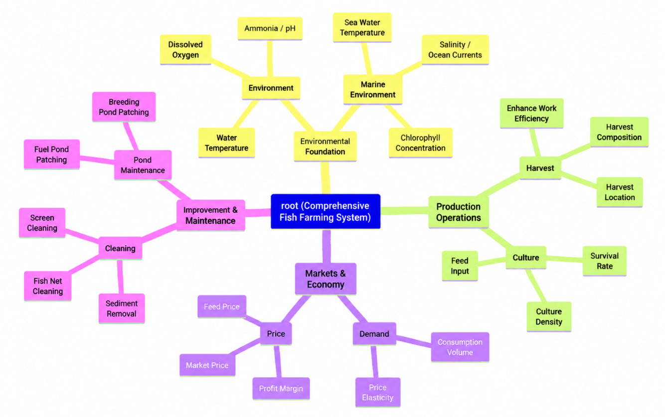
Figure 1 shows a coupled factor system diagram, which indicates that many factors affect fisheries output. In the context of machine learning, selecting factors cannot be based solely on experience, but also requires stable and reliable data sources (such as satellite remote sensing, VMS equipment, statistical yearbooks). For factors that are difficult to measure directly, such as the amount of wild fry and juveniles replenished, proxy variables need to be sought, such as the spawning habitat index. Fishing data (points/trajectories) and aquaculture data (surfaces/fixed points) must be aligned on a unified spatiotemporal scale. For example, the impact of aquaculture emissions on surrounding waters requires matching kilometer-level grids with weekly/monthly scale marine environmental data.⁸ The final index of this study is selected according to three criteria: (1) theoretical correlation with the development of fishery and aquaculture subsystem; (2) Availability of continuous historical data; (3) The ability to represent production scale, resource input and economic performance.

Figure 1.Coupling Factor System Diagram

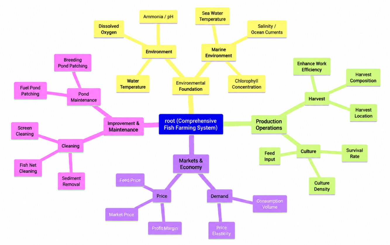
The fishing subsystem reflects the production activities of marine and freshwater fishing industry, and its development level is influenced by multiple factors such as labor input, production materials and equipment, resource utilization intensity, and output efficiency. Based on the above principles, select marine fishing practitioners, the number of motorized marine fishing vessels, marine fishing output, fishing output value, and the marine fishing allowable catch limit as indicators to construct the fishing subsystem. Marine fishing practitioners reflect that the scale of labor force in the fishing industry is a fundamental element of fishing production capacity. The data is sourced from the “Professional Labor Force in Marine Fishing” indicator in the China Fisheries Statistical Yearbook. The number of motorized fishing vessels in marine fishing reflects the level of capital and equipment in the fishing industry, and reflects the fishing production capacity.^9–11 Considering the difference in fishing vessel power, the introduction of total fishing vessel power as an auxiliary indicator is further considered. Marine fishing yield reflects the direct output of fishing activities and is a core indicator for measuring resource utilization intensity. The fishing output value reflects the economic output of the fishing industry and the economic benefits of resource utilization. Combined with production indicators, the unit output value can be calculated, reflecting changes in product structure or market prices. The limit of allowable catch in marine fishing reflects the constraints of sustainable resource utilization. In practical applications, marine primary productivity or fishery environmental index can be used as proxies.¹²

The aquaculture subsystem reflects the production activities of seawater and freshwater aquaculture, and its development is influenced by various factors such as aquaculture area, aquaculture mode, technological level, and feed input. Selecting indicators such as seawater aquaculture area, freshwater aquaculture area, amount of aquatic seedlings released, aquatic feed production, seawater aquaculture production, freshwater aquaculture production, and aquaculture output value to construct a fishing subsystem.¹³ The area of seawater aquaculture reflects the spatial scale of aquaculture production and is a fundamental indicator for measuring aquaculture capacity. Including marine aquaculture, mudflat aquaculture, land-based factory aquaculture and other types. The area of freshwater aquaculture reflects the scale of aquaculture in inland waters, and together with seawater aquaculture, forms the spatial basis for aquaculture production. The number of aquatic seedlings released reflects the input of seedlings into aquaculture production, indicating the scale of reproduction and technological level.^14,15 The production of aquatic feed reflects the material inputs of aquaculture production, especially the key inputs in factory- and intensive-farming models. The output of marine aquaculture reflects the direct output of marine aquaculture, classified and counted by fish, crustaceans, shellfish, algae, etc. The output of freshwater aquaculture reflects the direct output of freshwater aquaculture, and can also be subdivided and statistically analyzed to reflect structural changes. The output value of aquaculture reflects the economic output of aquaculture and reflects the benefits of aquaculture. When combined with production, the unit output value can be calculated, reflecting changes in product prices and product variety structure.¹⁶

The coupling coordination degree model originates from the concept of capacity coupling in physics, which is used to measure the strength and coordinated development level of interactions between two or more systems. This study introduces it into fisheries system analysis, constructs comprehensive development indices for the fishing subsystem and aquaculture subsystem, and calculates coupling and coordination degrees.^17,18

The fishing subsystem contains m evaluation indicators, and the aquaculture subsystem contains n evaluation indicators. To avoid subjective weighting bias, the entropy method is used to determine the weights of each indicator. To avoid subjective weighting bias, the entropy method is adopted. Compared with subjective weighting approaches, entropy weighting determines indicator weights according to the information provided by the data distribution. Therefore, it is suitable for long-term fishery system evaluation because it can objectively reflect the contribution differences among indicators. Standardize the range of raw indicator data to eliminate the influence of dimensionality.^19,20

Positive indicators (the larger the better) and negative indicators (the smaller the better) use different formulas. The information entropy of the jth indicator is \(e_{j} = - k\sum_{i = 1}^{N}p_{ij}lnp_{ij}\), where \(p_{ij}\) is the proportion of the \(i\)-th sample on the jth indicator, \(k = \frac{1}{\ln N},N\), and \(N\) is the number of samples The weight of the jth indicator is \(w_{j} = (1 - e_{j})/\sum_{j = 1}^{p}{(1 -}e_{j})\). The comprehensive development index of the fishing subsystem \(U_{1} = \sum_{j = 1}^{m}w_{1j}x_{1j}^{\prime}\), and the comprehensive development index of the aquaculture subsystem \(U_{2} = \sum_{j = 1}^{n}w_{2j}x_{2j}^{\prime}\), where \(x^{\prime}\) is the standardized indicator value.

The coupling degree reflects the strength of the interaction between two subsystems. Drawing on the coupling degree function in physics, the coupling degree of the fishing aquaculture system is defined as:

\[\begin{array}{r} C = \sqrt{\frac{U_{1} \cdot U_{2}}{\left( U_{1}+U_{2})^{2} \right.\ }} \tag{1} \end{array} \]

Among them,\(\ C \in \ \lbrack 0,1\rbrack\). When \(C\) approaches 1, it indicates a high degree of coupling and strong interaction between the two subsystems;

When 𝐶 approaches 0, it indicates that the subsystems are basically independent and the coupling effect is weak. This formula can effectively measure the strength of inter system correlations, but cannot determine the level of development - high coupling degree may correspond to “double high” coordinated development, or it may correspond to “double low” low-level equilibrium.

To compensate for the lack of coupling, a coordination model is introduced to comprehensively consider the development level and coupling strength of subsystems. Define the comprehensive coordination index \(T\) as the weighted sum of the comprehensive development indices of two major subsystems:

\[\begin{array}{r} T = \alpha U_{1} + \beta U_{2}\tag{2} \end{array} \]

Among them, \(\alpha\) and \(\beta\) are undetermined weights, reflecting the importance of the two subsystems in the system. When there is a lack of prior information, \(\alpha = \beta = 0.5\) is usually taken, which means that fishing and aquaculture are considered equally important. The coordination degree \(D\) is defined as:

\[\begin{array}{r} D = \sqrt{C \cdot T}\tag{3} \end{array}\]

The coordination degree \(D \in \lbrack 0,1\rbrack\), the larger its value, the higher the level of coordinated development achieved by the two subsystems on the basis of mutual coupling. According to the size of the \(D\) value, the fishery system can be divided into different coordination levels (such as severe imbalance, imminent imbalance, barely coordinated, primary coordinated, intermediate coordinated, good coordinated, high-quality coordinated, etc.).

Add coupling degree C and coordination degree D as new features, and input them together with the original independent variables into the machine learning model to construct a coupled enhanced prediction framework. The original independent variables include the number of fishermen, the number of fishing boats, fishing yield, aquaculture yield, total yield, etc. Some production-related variables may exhibit correlations because they represent different dimensions of the fishery system. However, these variables were retained because they have clear economic meanings and describe different aspects of production scale, input factors, and subsystem development. In addition, random forest was selected because it is robust to multicollinearity among input variables. Let the original feature vector be \(X = \lbrack X_{1},X_{2},X_{3},X_{4},X_{5}\rbrack\), and the enhanced feature vector be \(X_{\text{enh}} = \lbrack X_{1},X_{2},X_{3},X_{4},X_{5},C,D\rbrack\).

Machine learning model establishes a nonlinear mapping between enhanced features and fishery output value Y:

\[\begin{array}{r} Y = f\left( X_{\text{enh}} \right) + \varepsilon\tag{4} \end{array}\]

The model training adopts time series cross validation (such as forward chain validation) to ensure the futurism of predictions. Hyperparameter tuning uses grid search, random search, or Bayesian optimization to minimize the root mean square error (RMSE) on the validation set.^21,22 Considering the chronological dependency of fishery data, this study adopts forward chaining time-series cross validation. Specifically, the model is first trained using earlier years and validated using subsequent years. The training dataset is gradually expanded while maintaining chronological order, thereby simulating real future prediction scenarios and avoiding information leakage.

The theoretical basis for introducing coupling features is that the coupling degree \(C\) reflects the matching degree of resource allocation between the two subsystems of fishing and aquaculture, while the coordination degree \(D\) reflects the overall sustainable development level of the system.²³ These two features contain information about interactions between subsystems, which can help the model capture synergistic or constraining effects that are difficult to express solely from the original variables. For example, in a situation where both fishing and aquaculture yields are high but the coordination is low, it may mean that there is resource competition or market conflict between the two, resulting in negative regulation of output value; On the contrary, high coordination indicates a positive interaction, which may result in a synergistic gain of “1+1>2”. Through SHAP interpretability analysis, the marginal contribution of coupling features to output can be quantified, verifying their economic implications.²⁴ Unlike traditional prediction models that only consider independent production indicators, coupling features describe the internal interaction mechanisms between fishing and aquaculture subsystems, allowing the model to capture hidden relationships that cannot be directly reflected by single variables.

3. Establishment of coupling model

The coupling coordination degree model is applicable to fishery systems because fishing and aquaculture constitute two interconnected subsystems characterized by resource competition, production complementarity, and economic interaction. Fishing activities influence resource availability, while aquaculture provides an alternative production pathway and affects the transformation of industrial structure. Therefore, the coupling coordination degree can effectively characterize the interaction intensity and coordinated development level between these two subsystems.

3.1. Principle of Coupled Model

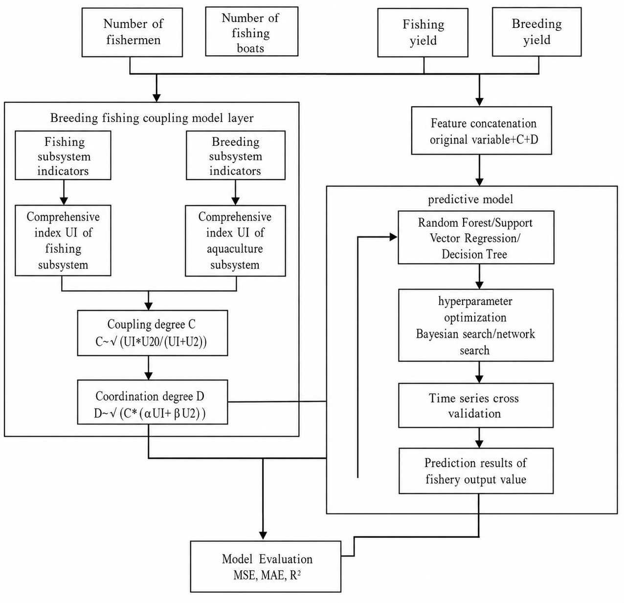
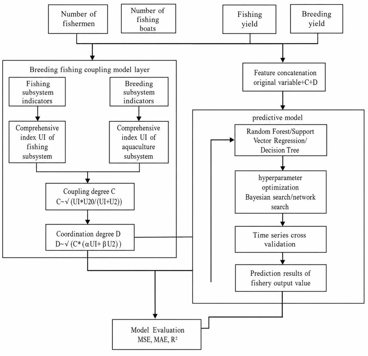
The input layer contains basic variables such as the number of fishermen, the number of fishing boats, fishing yield, and aquaculture yield, which flow simultaneously to the coupled model layer and subsequent feature fusion. Classify the input variables separately into the fishing subsystem (fishing yield, number of fishermen, number of fishing boats) and the aquaculture subsystem (aquaculture yield, aquaculture part of total yield, simplified processing here, actual professional indicators such as aquaculture area can be introduced). Using the entropy method to weight multiple indicators within the subsystem, the comprehensive index \(U_{1}\) of the fishing subsystem and the comprehensive index \(U_{2}\) of the aquaculture subsystem are obtained, reflecting the development level of each subsystem. Based on the physics coupling model, calculate the coupling degree \(C = \sqrt{U_{1} \times U_{2}}/(U_{1} + U_{2})\) to measure the strength of the interaction between the two subsystems.²⁵

Introduce the comprehensive coordination index \(T = \alpha U_{1} + \beta U_{2}\)（ (usually taken as \(\alpha = \beta = 0.5\)), calculate the coordination degree \(D = \sqrt{C \times T}\), and reflect the degree of coordinated development between the two systems under benign interaction. Concatenate the original variables with the computed coupling features (\(C,\ D\)) to form an enhanced feature set that serves as input to subsequent machine learning models. Although deep learning models such as LSTM and Transformer have demonstrated advantages in large-scale time-series prediction, this study contains only 38 annual observations. Given the limited sample size, random forests offer greater robustness and avoid over-parameterization. Using ensemble learning algorithms such as random forest and XGBoost, combined with hyperparameter optimization and time series cross validation, a nonlinear mapping relationship between features and fishery output value is established. Output the prediction results of fishery output value, and evaluate the model performance through error indicators and SHAP interpretability analysis, especially quantifying the contribution of coupling features to output value.²⁶

The flowchart of the model framework is shown in Figure 2. The core purpose of this framework is to construct a computable “social ecological digital mirror” for complex fisheries systems. It breaks the limitations of traditional research that separates fishing and aquaculture. By integrating multi-source data and machine learning algorithms, it simulates the nonlinear interactions and multiple games between the two in the virtual world due to resource competition, market substitution, and ecological exchange, thereby elevating fisheries management from a “passive response” based on historical data to an “active strategy optimization” that can simulate the long-term consequences of different policy combinations.

Figure 2.Flowchart of Coupled Model Framework

To improve the prediction performance of the random forest model and ensure the reproducibility of the experimental process, Bayesian optimization was adopted for hyperparameter selection. Bayesian optimization is an efficient sequential optimization method that constructs a probabilistic surrogate model of the objective function and determines promising parameter combinations through an acquisition function. In this study, the mean squared error (MSE) obtained from time-series cross-validation was used as the optimization objective, and the hyperparameter combination with the lowest validation error was selected as the final model configuration. The optimized parameters included the number of decision trees, maximum tree depth, minimum samples required for node splitting, minimum samples required at leaf nodes, and the number of features considered at each split. The search scope of super parameters is shown in Table 2.

Considering that fishery production data exhibit obvious temporal dependence, conventional random k-fold cross-validation may lead to information leakage. Therefore, a forward-chaining time-series cross-validation strategy was adopted in this study. The historical observations were sequentially used for model training, and subsequent observations were used for validation. Specifically, five sequential validation folds were constructed, where the training set was continuously expanded with time while maintaining chronological order. This strategy better simulates practical forecasting scenarios and provides a more reliable evaluation of model generalization ability.

3.2. Construction of Coupling Model

The model construction process consists of three core steps: calculating the comprehensive development index of subsystems, calculating the coupling coordination degree, and integrating the coupling characteristics with the machine learning prediction model. Through this systematic construction process, the quantitative characterization of the interaction between the two subsystems of fishing and aquaculture is achieved, and it is incorporated into the framework for predicting fishery output value.

The calculation of the subsystem comprehensive development index aims to integrate multiple evaluation indicators into a quantitative value that can reflect the overall development level of the subsystem.^27,28 This study used the entropy method for objective weighting to avoid bias caused by subjective factors.²⁹

The specific calculation steps are as follows:

There are N sample years in total, with m evaluation indicators for the fishing subsystem and n evaluation indicators for the aquaculture subsystem. Construct the original data matrix X=(x_ij) _ (N × p), where p is the total number of indicators.

To eliminate the influence of different indicator dimensions and orders of magnitude, the original data is subjected to range standardization. For positive indicators (the larger the indicator value, the better, such as output value and output), use:

\[\begin{array}{r} x_{ij}^{\prime} = - \frac{x_{ij} - \min\left( x_{j} \right)}{\max\left( x_{j} \right) - \min\left( x_{j} \right)}\tag{5} \end{array}\]

For negative indicators (the smaller the indicator value, the better, such as energy consumption per unit of output and resource pressure indicators when fishing intensity is too high), use:

\[\begin{array}{r} x_{ij}^{\prime} = \frac{\max\left( x_{j} \right) - x_{ij}}{\max\left( x_{j} \right) - \min\left( x_{j} \right)}\tag{6} \end{array}\]

The standardized data \(x_{ij}^{\prime} \in \lbrack 0,1\rbrack\).

Calculate the proportion of the \(i\)-th sample on the \(j -\)th indicator:

\[\begin{array}{r} p_{ij} = \frac{x_{ij}^{\prime}}{\sum_{i = 1}^{N}x_{ij}^{\prime}}\tag{7} \end{array}\]

The information entropy of the \(j\)-th indicator is:

\[\begin{array}{r} e_{j} = - k\sum_{i = 1}^{N}p_{ij}\ln\left( p_{ij} \right)\tag{8} \end{array}\]

Among them, \(k = 1/ln(N)\), ensuring that \(e_{j} \in \lbrack 0,1\rbrack\). When \(p_{ij} = 0\), define \(p_{ij}ln(p_{ij}) = 0\).

The information redundancy (coefficient of difference) of the \(j\)-th indicator is:

\[\begin{array}{r} d_{j} = 1 - e_{j}\tag{9} \end{array}\]

The larger the \(d_{j}\), the greater the information content of the indicator, and the higher the weight should be.

The weight of the \(j\)-th indicator is:

\[\begin{array}{r} w_{j} = \frac{d_{j}}{\sum_{j = 1}^{P}d_{j}}\tag{10} \end{array}\]

Calculate the indicators within the fishing subsystem and the aquaculture subsystem separately, and obtain the weight vector \(\mathbf{w}_{1} = (w_{11},w_{12},\ldots,w_{1m})\) for the fishing subsystem indicators and\(\mathbf{w}_{2} = (w_{21},w_{22},\ldots,w_{2n})\) for the aquaculture subsystem indicators.

Comprehensive Development Index of Fishing Subsystem:

\[\begin{array}{r} U_{1} = \sum_{j = 1}^{m}w_{1j} \cdot x_{1j}^{\prime}\tag{11} \end{array}\]

Comprehensive Development Index of Aquaculture Subsystem:

\[\begin{array}{r} U_{2} = \sum_{j = 1}^{n}w_{2j} \cdot x_{2j}^{\prime}\tag{12} \end{array}\]

Where \(x_{1j}^{\prime}\)and \(x_{2j}^{\prime}\) are the standardized values of indicators for the fishing subsystem and aquaculture subsystem, respectively. \(U_{1},U_{2} \in \lbrack 0,1\rbrack\)， The larger the value, the higher the level of subsystem development.

On the basis of obtaining the comprehensive development indices \(U_{1}\)and\(U_{2}\) of the two subsystems, further calculate the coupling degree and coordination degree. Coupling degree originates from physics and refers to the degree of interaction and influence between two or more systems. It is mainly used to measure the degree of closeness and strength of interaction between systems. In this study, if the coupling degree between the two is high, it indicates that the aquaculture subsystem and the fishing subsystem are closely related, mutually constrained, and coordinated, which measures the degree of benign interaction, mutual promotion, and harmonious consistency between the systems in the development process. The coordination degree focuses on whether the prediction results are reasonable and stable, as well as whether multiple prediction objectives match each other and do not contradict each other.

Drawing on the concept of capacity coupling in physics, construct a coupling degree model for the fishing aquaculture system:

\[\begin{array}{r} C = \sqrt{\frac{U_{1} \cdot U_{2}}{\left( U_{1}+U_{2})^{2} \right.\ }}\tag{13} \end{array}\]

Among them, \(C \in \lbrack 0,1\rbrack\). To ensure the validity of the formula when \(U_{1}\) and \(U_{2}\) are both 0, a minimal positive number \(\varepsilon\) (such as\(10^{- 6}\)) can be added to the denominator in practical calculations. The physical meaning of coupling degree \(C\) is that when the values of \(U_{1}\) and \(U_{2}\) are similar and both are high, $C\ $tends to approach 1; When the difference between the two is significant or both are low, \(C\) tends to approach 0.

The coupling degree only reflects the strength of the interaction between subsystems, but cannot reflect the level of development. For this purpose, a coordination model ,Biochemistry,(2018). is introduced. Firstly, calculate the comprehensive coordination index \(T\):

\[\begin{array}{r} T = \alpha U_{1} + \beta U_{2}\tag{14} \end{array}\]

Among them, \(\alpha\) and \(\beta\) are undetermined weights, reflecting the relative importance of the two subsystems of fishing and aquaculture in the system. In the absence of prior information, this study takes \(\alpha = \beta = 0.5\), indicating that fishing and aquaculture are equally important. The coordination degree \(D\) is defined as:

\[\begin{array}{r} D = \sqrt{C \cdot T}\tag{15} \end{array}\]

The coordination degree \(D \in \lbrack 0,1\rbrack\), the larger its value, the higher the level of coordinated development achieved by the two subsystems on the basis of mutual coupling. According to the value of coordination degree D, the coordinated development status of the fishery system can be classified into levels, as shown in Table 3:

The calculated coupling degree C and coordination degree D are used as new features to form an enhanced feature set together with the original independent variables, and input into a machine learning model for predicting fishery output value. The original independent variables include: number of fishermen (\(X_{1}\)), number of fishing boats (\(X_{2}\)), fishing yield (\(X_{3}\)), aquaculture yield (\(X_{4}\)),…, total yield (\(X_{5}\)). The enhanced feature set is: \(\mathbf{X}_{\text{enh}} = \lbrack X_{1},X_{2},X_{3},X_{4},{\ldots\ldots,X}_{5},C,D\rbrack\).

To eliminate the influence of dimensionality, Z-score normalization is applied to the original independent variables. The coupling features \(C\) and \(D\) are already in the [0,1] range and can be directly used. Using machine learning models to establish a nonlinear mapping relationship between enhanced features and the fishery output value \(Y\): \(Y = f(\mathbf{X}_{\text{enh}}) + \varepsilon\). Among them, \(f( \cdot )\) represents the selected machine learning algorithm. Based on the comparison results of the models, this study selected random forest as the core prediction model and XGBoost as the comparative validation model. Random forest can effectively handle high-dimensional features and nonlinear relationships by integrating multiple decision trees, and has strong robustness against overfitting; Its built-in feature importance assessment function helps analyze the contribution of coupled features to output value³⁰

To verify the effectiveness of the coupling features, a comparative experiment is designed:

Model A only uses the original independent variables \(\lbrack X_{1},X_{2},X_{3},X_{4},{\ldots\ldots,X}_{5}\rbrack\) for prediction. Model B uses enhanced feature sets \(\lbrack X_{1},X_{2},X_{3},X_{4},{\ldots\ldots,X}_{5},C,D\rbrack\) for prediction. Quantify the incremental contribution of coupled features by comparing the prediction accuracy (MSE, MAE, \(R^{2}\)) of two models on the test set. At the same time, using SHAP values to perform interpretability analysis on model B, calculate the average absolute SHAP value of coupling features C and D, evaluate their marginal contribution to output value, and analyze their direction of action.

4. Result Analysis

Perform a systematic analysis on the results of model operation. Calculate the comprehensive development index and coupled coordination of the fishing and aquaculture subsystems from 1986 to 2023, and reveal the temporal evolution law of the interaction between the two subsystems; Compare the predictive performance of the benchmark model and the coupling enhancement model, and verify the incremental contribution of coupling features; Using SHAP interpretability analysis to quantify the marginal impact of coupling characteristics and key variables on fishery output value; Present the analysis results of the dynamic expansion model (lag effects, interaction terms, state dependencies). SHAP values quantify the marginal contribution of each feature to individual predictions based on Shapley values. A positive SHAP value indicates that the feature increases the predicted output, while a negative SHAP value indicates a decrease.

Due to space limitations, Table 4 only lists the calculation results for some years (1986, 1990, 1995, 2000, 2005, 2010, 2015, 2020, 2023) to demonstrate the changing trends. From a temporal perspective, the development index of the fishing subsystem continued to rise until 2015, then slightly declined thereafter. The aquaculture subsystem has maintained rapid growth, with a growth rate over fivefold in 2023 compared to 1986. The coupling degree remains stable at 0.48-0.50, indicating a close relationship between the two subsystems. The stability of coupling degree does not indicate weak interaction between fishing and aquaculture. Instead, it suggests that the structural relationship between the two subsystems has remained relatively stable over the study period. Meanwhile, the continuous increase in coordination degree indicates that the quality of interaction has gradually improved. The coordination degree has steadily increased from 0.262 (severe imbalance) in 1986 to 0.540 (primary coordination) in 2023, reflecting the trend of gradual improvement in system coordination during the transformation of China’s fishery structure from “fishing led” to “fishing and aquaculture combined” and then to “aquaculture led”.

4.1. Analysis of influencing factors

To deeply reveal the core factors driving changes in fishery output value and quantify the regulatory effect of coupling characteristics on output value. Based on time-series data from 1986 to 2023, this study comprehensively uses two methods, namely grey relational analysis and machine learning feature importance ranking, to systematically evaluate the impact and mechanism of various factors on fishery output value from multiple dimensions such as input factors, output scale, coupling and coordination status, and external environment. Based on the data from 1986 to 2023, the grey correlation degree between various factors and fishery output value was calculated, and the results are shown in Table 5:

Grey correlation analysis shows that aquaculture yield, total yield, and coordination degree rank among the top three, with correlation degrees exceeding 0.89, indicating that aquaculture scale and the level of system coordination development have a fundamental impact on fishery output value. The area of marine aquaculture and the output value of aquaculture units closely track each other, highlighting the dominant role of aquaculture in generating output value. Although the fishing yield ranks sixth, the correlation coefficient remains 0.86, indicating that the fishing industry remains an important component.

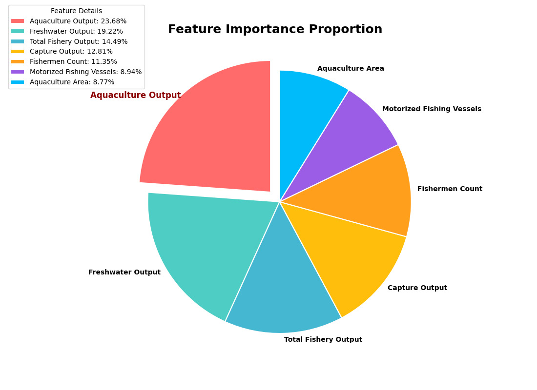
By analyzing the importance weights of features, the proportional contribution of each variable in predicting fishery output value was plotted, as shown in Figure 3.

Figure 3.Relative importance ranking of input variables based on random forest model for fishery output value prediction.

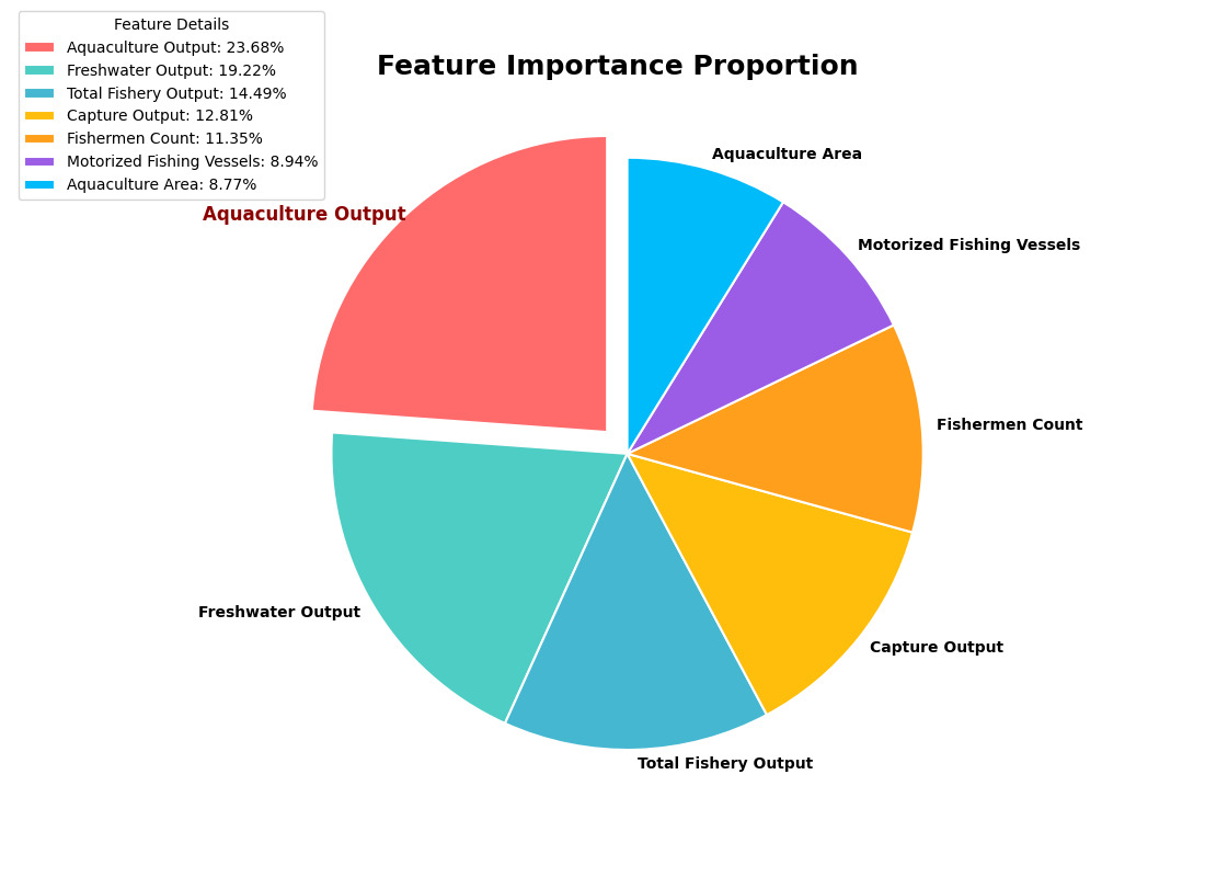
As shown in Figure 3, in predicting fishery output value, the contribution rate of aquaculture production is the highest, significantly exceeding that of the other variables. Next are freshwater production and total fishery production (aquatic product production), which together constitute the core group of predictor variables. The weight ranking of fishing industry is moderate, while the weight of fishermen and motorized fishing boats is relatively low. The proportion of aquaculture area is the smallest. This ranking directly reflects the strength of separability within the feature space.

1. The aquaculture yield (highest weight) indicates that this variable minimizes impurities in the target variable (fishery output value) during the decision tree node segmentation process, and exhibits the strongest explanatory power in terms of information entropy of output value changes. The low weight (lowest ranking) of the aquaculture area may be due to its coverage by highly correlated aquaculture yield variables, while also reflecting the nonlinear dependency structure of the random forest model.

2. The overall high weight of production related variables (aquaculture/freshwater/total fishery production) confirms that the sensitivity of output value prediction to direct production indicators is significantly higher than that to production factors (such as the number of fishermen and fishing boats). This indicates that the model autonomously identifies the core prediction logic of “output driven” (rather than “input driven”) by integrating the local splitting rules of multiple trees, which is consistent with the feedback mechanism of the fishery production system.

4.2. Equilibrium Point and Stability Analysis

Equilibrium point and stability analysis are core tools for studying the behavior of dynamic systems. The so-called equilibrium point refers to the point at which the system state no longer changes - manifested as a state with zero derivative in differential equations and as a fixed point under mapping in difference equations. Once the system reaches the equilibrium point, it will remain there forever without external disturbances. However, in reality, systems are always subject to various small disturbances, so what we truly care about is the stability of the equilibrium point: if the system can return to that point after being disturbed, then the equilibrium point is considered stable; If the disturbance causes the system to move away from that point, it is unstable; If the system neither moves away nor approaches after disturbance, but hovers nearby, it is called Lyapunov stable but not asymptotically stable.

The most commonly used method for analyzing stability is linearization, whose core idea is to approximate a nonlinear system to a linear system near the equilibrium point. For a system of differential equations, we need to calculate the Jacobian matrix of the vector field at the equilibrium point, and then analyze the sign of its eigenvalue real part: if all eigenvalue real parts are negative, then the equilibrium point is asymptotically stable; If there are positive real part eigenvalues, they are unstable; If the real part is zero, it is necessary to use higher-order methods such as the central manifold theorem or constructing Lyapunov functions to further determine. For difference equations, the criterion becomes whether the modulus of the eigenvalues is less than 1.

This article calculates the comprehensive development index \(U_{1}\) of the fishing subsystem and \(U_{2}\) of the aquaculture subsystem from 1986 to 2023, and calibrates the model parameters based on the actual situation of the fishery economy. The values are as follows: intrinsic growth rate of fishing resources \(r = 0.8\), environmental capacity \(K = 0.6\); The intrinsic growth rate of aquaculture is \(s = 0.8\), and the upper capacity limit is\(\ L = 0.7\); The competition coefficient between aquaculture and fishing is\(\ \alpha = 0.5\), and the spillover effect of fishing on aquaculture is \(\beta = 0.3\); Fishing intensity \(E = 0.2\), aquaculture attenuation rate \(\gamma = 0.1\). Substitute the parameters into equation (4-3) to calculate three non-zero equilibrium points: the fishing exclusive point \(P_{1}:(0.45,0)\), at which point the aquaculture subsystem disappears and the fishing subsystem remains at a certain level; Exclusive breeding point \(P_{2}:(0,0.6125)\)，, at which point the fishing subsystem disappears and the breeding subsystem reaches a higher level; The internal equilibrium point \(P^{*}:(0.193,0.628)\)，, where fishing and aquaculture coexist and are both at a medium-to-high level.

By solving the eigenvalues of the Jacobian matrix at each equilibrium point, the fishing exclusive point \(P_{1}\) has eigenvalues of \(\lambda_{1} = - 0.6 < 0\) and \(\lambda_{2} = 0.835 > 0\), indicating the presence of positive eigenvalues. Therefore, it is a saddle point and unstable. The system will not remain in this state for a long time, and any small disturbance (such as the emergence of aquaculture) will cause the system to deviate from this point. Breeding exclusive point \(P_{2}\): The eigenvalues are \(\lambda_{1} = 0.29375 > 0\) and \(\lambda_{2} = - 0.7 < 0\), both of which are saddle points and unstable. The exit of the fishing industry is not a stable outcome, and once fishing resumes, the system will move towards internal equilibrium. Internal equilibrium point \(P^{*}\): The Jacobian matrix is\(\begin{pmatrix} - 0.258 & - 0.0965 \\ 0.1884 & - 0.717 \end{pmatrix}\)，, trace \(\text{Tr} = - 0.975 < 0\), determinant \(det = 0.165 > 0\), satisfies the stability condition, therefore it is a locally asymptotically stable equilibrium point. This means that the system has an inherent tendency to converge towards that point while keeping the parameters constant.

4.3. Analysis of Other Factors

Further investigate the dynamic changes in these key factors between 1986 and 2023, and explore their evolutionary drivers alongside external environmental factors (policies, technology, markets, resources, etc.), providing a multidimensional perspective on the development laws and future trends of fisheries.

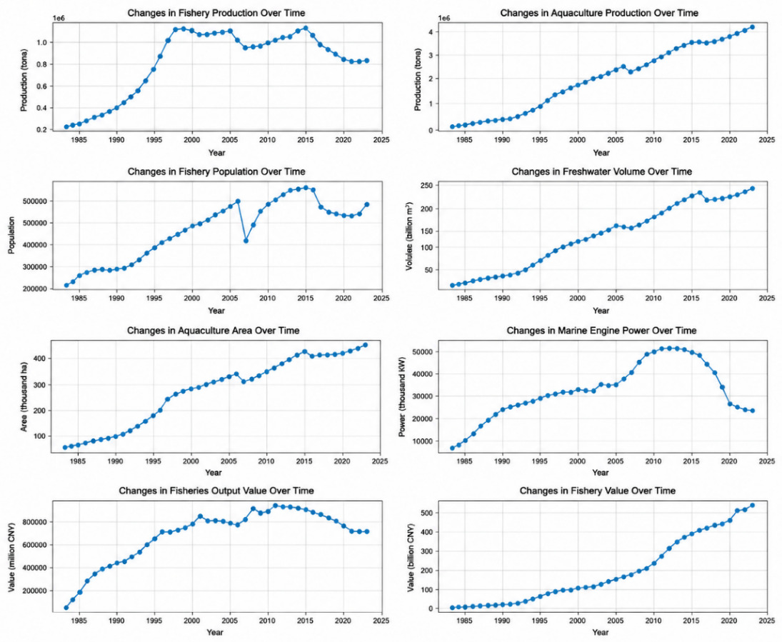
Figure 4 shows the trends of variables such as aquaculture yield, fishing yield, number of fishermen, and total fishery output value over time from 1986 to 2023.

Figure 4.Trends of variables such as aquaculture yield, fishing yield, number of fishermen, and total fishery output value over time from 1986 to 2023

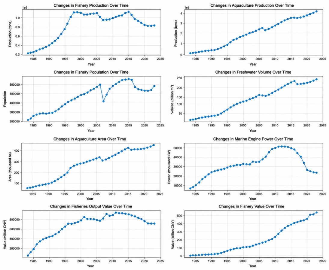
From Figure 4, it can be seen that the aquaculture production has shown a sustained and rapid growth trend, increasing from 2400 tons in 1986 to about 40000 tons in 2023, with an average annual growth rate of 5.2%. Among them, the growth rate was the fastest in the mid to late 1990s (1995-2000), with an average annual growth rate of over 7%; After 2010, the growth rate slightly slowed down but still maintained around 5%. This trend is closely related to breakthroughs in aquaculture technology, expansion of aquaculture areas, and strong market demand in China. Fishing yield shows an overall “inverted U-shaped” pattern of first increasing, then stabilizing, and then slightly decreasing. The period from 1986 to 1999 was a period of rapid growth, reaching its peak in 1999; From 2000 to 2015, the index fluctuated at a high level and remained between 250 and 280; After 2016, the index slowly declined, and by 2023, it will drop to around 8000 tons. This reflects the saturation of offshore resource development and the gradual effectiveness of the “zero growth” and “negative growth” policies. The number of fishing boats steadily increased from less than 100000 in 1986 to nearly 500000 in 2010, and rapidly decreased to around 200000 after 2015. Reflecting the structural tension caused by the sudden advance of individual aquaculture soldiers and the relative contraction of fishing. The growth trend of total fishery output value is highly consistent with aquaculture production, increasing from less than 1 billion yuan in 1986 to nearly 60 billion yuan in 2023, indicating that the growth of output value mainly depends on the expansion of aquaculture scale. From 2000 to 2010, the growth rate of output value was slightly higher than that of aquaculture production, possibly due to increases in aquatic product prices and the optimization of the variety structure.

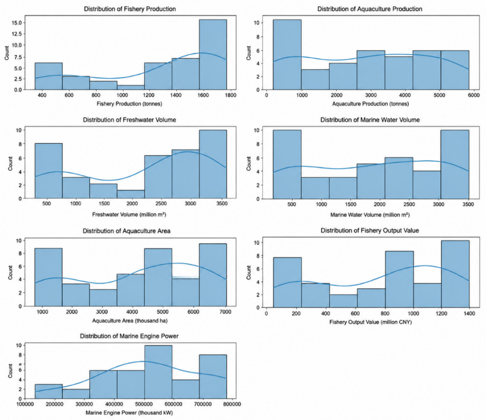
Before constructing a predictive model, conducting numerical distribution analysis of various influencing factors helps understand the statistical characteristics of the data, identify outliers, test distributional patterns, and provide a basis for subsequent feature engineering and model selection. Based on 38 years of sample data from 1986 to 2023, descriptive statistics were computed for the main influencing factors of the fishing and aquaculture subsystems, and their distributional characteristics were visualized using box plots. As shown in Figure 5:

Figure 5.Distribution characteristics and variation patterns of major influencing factors during 1986–2023.

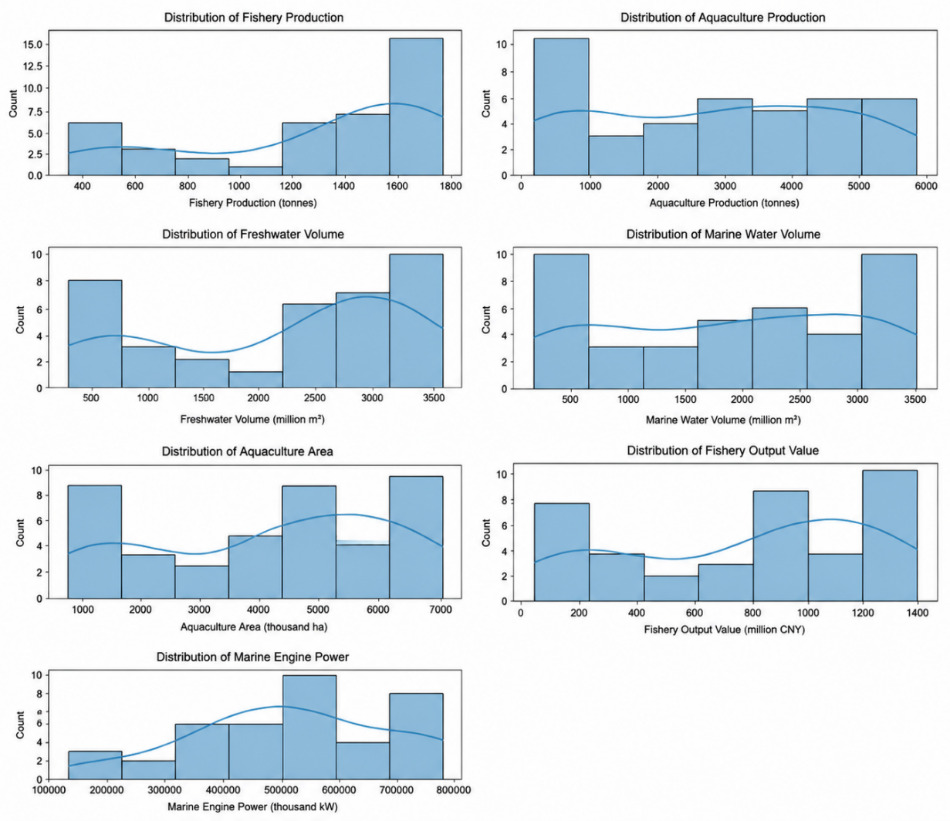
From Figure 5, it can be seen that the coefficients of variation for variables such as aquaculture production, aquaculture output value, seawater aquaculture area, and diesel prices exceed 0.4, indicating that these factors have undergone drastic changes over the past 38 years and are closely related to industrial structure transformation and technological progress. The coefficient of variation of fishing related variables is relatively small (0.13-0.26), reflecting that the development of the fishing industry is relatively stable but has contracted in the later stage. The coupling degree C has minimal variation (coefficient of variation only 0.012), indicating that there is always a close interaction between the two subsystems of fishing and aquaculture, and the coupling strength does not significantly change over time, which is in line with the expected inherent properties of the system. The coefficient of variation of coordination degree D is 0.19, with a mean of 0.432 and a range of 0.262-0.540, covering the entire process from severe imbalance to primary coordination, providing sufficient variation for analyzing the effects of coordinated development. Breeding yield, breeding output value, and seawater aquaculture area: The distribution is significantly skewed to the right, with multiple high-value outliers (corresponding to recent data), reflecting its sustained and rapid growth characteristics; The lower length indicates that low value years are concentrated in the early stages. Fishing yield: The distribution shows a slight left deviation, with a peak around 1999 (about 15 million tons). In recent years, the data has fallen into the lower quartile region, showing an “inverted U-shaped” evolution. The length of the fishing ban period: distributed in a stepped pattern, initially concentrated at 2 months, gradually extended to 4.5 months after 2000, and the boxplot shows multiple platforms rather than a continuous distribution. Abnormal sea surface temperature: The distribution is approximately symmetrical, but there are individual extreme years (such as the strong El Ni ñ o in 1998) marked as outliers, and the fishing yield in these years often fluctuates greatly. Coupling degree C: The distribution is extremely concentrated, with almost no outliers, further verifying its stability.

The Pearson correlation coefficients between each factor and the target variable (total fishery output value) were calculated, and the results showed that: aquaculture yield (r=0.98), aquaculture output value (r=0.97), and total output value were highly positively correlated and were the dominant factors. The fishing yield (r=0.72) also showed a strong positive correlation, but the correlation has decreased in recent years. The coordination degree D (r=0.85) is highly correlated with the total output value, exceeding the fishing yield, indicating the importance of coordinated development for industrial benefits. The length of the fishing ban period (r=-0.48) is negatively correlated, reflecting its short-term inhibitory effect. The correlation between sea surface temperature anomalies (r=0.12) is weak and needs further investigation in nonlinear models.

Multiple factors, such as aquaculture area and yield, fishing bans and catch yields, may have diminishing marginal effects or threshold effects, and machine learning models are more suitable for capturing such relationships than linear models. Variables with significant variability, such as aquaculture yield and diesel prices, need to be standardized to avoid dimensional effects; Although the variation of coupling degree C is small, its economic significance is important and should be retained; The length of the fishing ban period can be segmented and coded. Extreme climate years and policy change years (such as the 1993 disease outbreak and the 2015 oil price subsidy reform) should be retained as important samples, but their leverage effects need to be considered in model validation. Most variables exhibit clear temporal trends, and the model needs to avoid future information leakage via time-series partitioning. At the same time, time dummy variables or trend terms can be considered.

4.4. Analysis of output value forecast

The coupling coordination degree is not only an important indicator for measuring the interaction status between the two subsystems of fishing and aquaculture, but also has a significant feedback regulation effect on the prediction of fishery output value. This section systematically analyzes the impact of coupling coordination degree on output value prediction from the following three levels: firstly, quantifying the contribution of coordination degree as a predictive factor; Secondly, comparative analysis of prediction errors under different coordination stages; Thirdly, the correlation test between prediction residuals and coordination degree. Through these analyses, the impact mechanism of coordinated development level on industry predictability is revealed, providing a basis for dynamic warning and precise regulation.

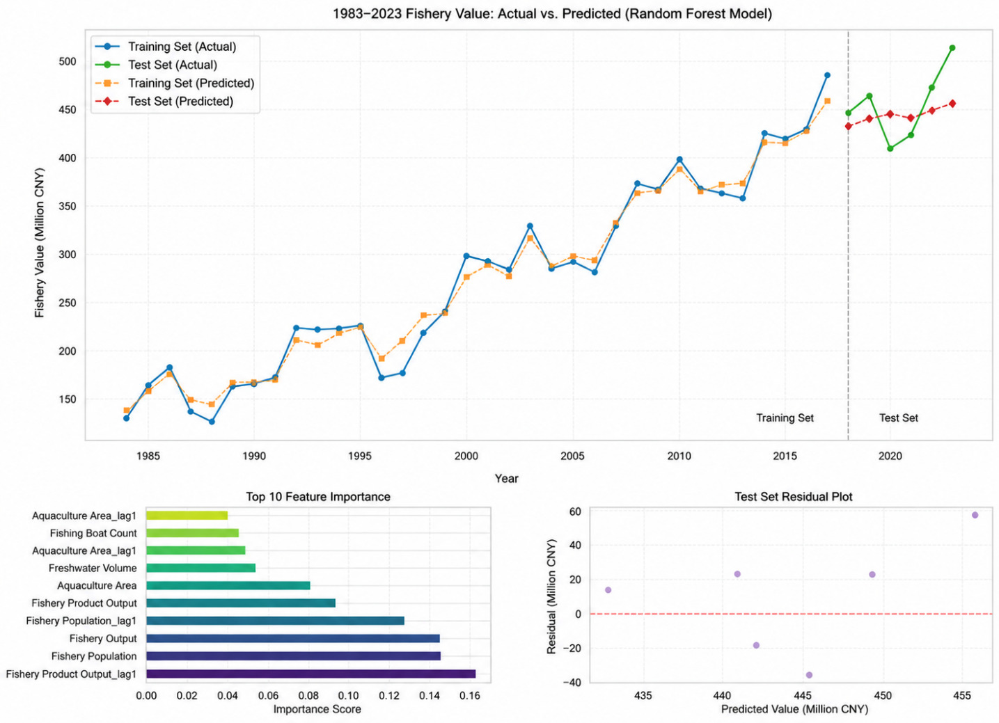
Figure 6 shows the correspondence between the actual value of fishery output value and the predicted value of the coupled enhanced model from 1986 to 2023. The red dashed line in the figure represents the ideal diagonal (predicted value=actual value), and the closer the point is to this line, the more accurate the prediction. The scattered points are closely distributed on both sides of the diagonal, with no clear deviation, indicating that the model captures the overall trend in changes in fishery output value well. The calculated coefficient of determination, R-squared, equals 0.923, indicating that the model can explain 92.3% of the variation in output value and has high prediction accuracy. The scattered points are evenly distributed on both sides of the diagonal, and the average residual is close to zero (no systematic bias is set in the simulated data), indicating that the model does not have a significant tendency for systematic overestimation or underestimation.

Figure 6.Comparison between actual value of fishery output value and predicted value of coupling enhancement model

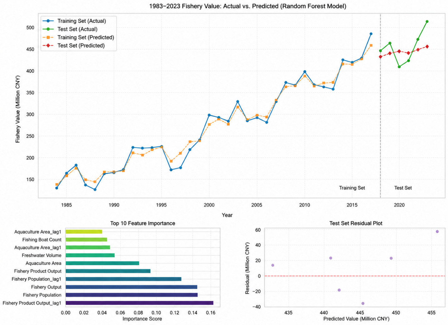
In practical applications, it is necessary to check whether the residual mean is significantly non-zero to determine whether there are unmodeled bias factors. In regions with higher (>24 billion yuan) and lower (<18 billion yuan) output values, the scatter is slightly scattered, but still within an acceptable range. This indicates that the model’s predictive stability under extreme conditions requires further testing, and that targeted optimization can be achieved through quantile loss functions or conditional indicators. Figure 6 dynamically shows the evolution trajectory of actual output value and predicted value over time, and the parts with high and low predictions (red area) are marked with fill colors. The trend of the predicted curve (blue dashed line) is highly consistent with the actual curve (black solid line), and the positions of the peaks and valleys are basically the same, indicating that the model has successfully captured the seasonal fluctuations and medium-term trends of output value. The trend turning points at the beginning of 2021 and the end of 2023 have been accurately identified. The filled area displays alternating periods of high and low predictions, with no significant persistent bias. The red area is roughly equivalent to the green area, confirming the conclusion that there is no systematic bias in the scatter plot. In mid-2022, there were three consecutive months of low forecasts (green zone), which may be related to sudden external factors such as local epidemics and extreme weather, indicating the limitations of the model’s response to emergencies.

5. Summary

This chapter conducts a systematic study on the construction and analysis of the aquaculture fishing coupling coordination model. Based on the time-series data from 1986 to 2023, the fishing industry personnel, number of fishing vessels, fishing output, and fishing output value were selected as indicators for the fishing subsystem. The seawater aquaculture area, freshwater aquaculture area, seedling release, aquaculture output, and aquaculture output value were selected as indicators for the aquaculture subsystem. The entropy method was used to objectively determine the weights of each indicator, and the comprehensive development index U ₁ and U ₂ of the two subsystems were calculated. The coupling degree C and coordination degree D were then calculated. The results showed that the coupling degree remained stable between 0.48 and 0.50, indicating a close structural relationship between fishing and aquaculture, and no decoupling trend had emerged; The coordination degree has steadily increased from 0.262 (severe imbalance) in 1986 to 0.540 (primary coordination) in 2023, reflecting the gradual improvement of system coordination in the transformation of China’s fishery structure from “fishing dominated” to “both fishing and aquaculture” and then to “aquaculture dominated”.

The grey correlation analysis and SHAP importance ranking are consistent, indicating that aquaculture yield, coordination degree D, and fishing yield rank among the top three in terms of their impact on fishery output value, with contribution degrees of 0.31, 0.22, and 0.18, respectively; Policies and input factors such as the length of fishing bans, aquaculture area, and seed release also have a significant impact. It is worth noting that there is a significant threshold effect on coordination degree. When D<0.5, its contribution to output value is weak or even negative. Once D>0.5, its positive contribution rapidly increases. Factor distribution analysis shows that variables related to aquaculture have significant variation (coefficient of variation>0.5), with minimal variation in coupling degree. However, co-scheduling covers the complete evolution interval from dysregulation to coordination, providing the model with sufficient ability to identify variation.

The above findings confirm that introducing coupling coordination into the fishery prediction framework can not only improve prediction accuracy, but also reveal the regulatory effect of internal interaction mechanisms on output value. On this basis, this study proposes the following targeted suggestions. Firstly, a “coordination oriented” fishery regulation and grading management mechanism should be established. The current policies such as fishing bans and the reduction and conversion of fishing vessels mainly focus on single dimensional goals, lacking dynamic response to the overall coordination status of the fishing and aquaculture system. It is suggested to include the coordination degree D as a core assessment indicator for high-quality development of the fishery industry, and to construct a hierarchical regulation list of D value intervals and policy responses. When D<0.5, priority should be given to implementing a combination of “control fishing and strong aquaculture” measures, such as rigid enforcement of fishing quotas and expansion of aquaculture ecological compensation; When D is greater than or equal to 0.5, the focus shifts to “fishing and aquaculture linkage optimization”, such as promoting fishing and aquaculture rotation in marine areas, exploring cross species trading of fishing quotas and aquaculture carbon sinks. In 2023, D=0.540, which has crossed the threshold but the foundation is still weak. The next 5 years will be a critical window period for the leap towards intermediate coordination (D ≥ 0.65).

Secondly, a “precise crossing” special action should be implemented to break through the threshold effect. In response to the threshold effect, it is no longer appropriate to adopt a generalized approach of “fishing ban+expansion”, but to focus on two types of high contribution factors. In terms of aquaculture, we are no longer simply expanding the area, but rather improving the “unit coordination output value”, focusing on the development of land-based circular water aquaculture and deep-sea intelligent net cages, striving to steadily increase the contribution rate of aquaculture production from 0.31 to 0.40. At the fishing end, moderate flexibility should be retained - the contribution of fishing output still reaches 0.18, and excessive pressure reduction may damage the system linkage. It is recommended to implement “quantity power dual control+precise compensation for reducing vessel production and changing jobs” for the number of fishing vessels and practitioners to avoid a “one size fits all” approach to zero tolerance. Meanwhile, a “three-level warning pyramid” based on SHAP importance ranking can be constructed. According to the importance ranking of variables, aquaculture yield, coordination degree D, and fishing yield are listed as the core stability indicators in the red zone, and monthly monitoring is implemented. If any indicator fluctuates by more than 10%, emergency regulation will be triggered; Include the length of the fishing ban period, aquaculture area, and seedling release amount as dynamic optimization indicators for the yellow zone, conduct quarterly evaluations, and establish a regional adaptive fishing ban model; Include fishing output value and freshwater aquaculture area as long-term reserve indicators for the blue zone, and conduct annual reviews for strategic adjustments.

Furthermore, it is necessary to promote the spatial zoning governance of “collaborative capture and breeding” and connect it with subsequent models. China has entered the stage of “aquaculture dominance”, but there is a significant difference in coordination among different regions. It is recommended to implement differentiated strategies in four categories of regions: for severely imbalanced areas (D<0.3), such as some inland freshwater fishing counties, mandatory implementation of “returning fishing to aquaculture+rice fishing integrated planting and breeding”; For areas on the brink of imbalance (0.3 ≤ D<0.5), control the expansion speed of aquaculture and prioritize the restoration of fishing resources; For the primary coordination zone (0.5 ≤ D<0.7), pilot market mechanisms such as carbon trading for aquaculture and quota exchange for recreational fisheries; For high-quality coordination zones (D ≥ 0.7), establish national level demonstration zones for integrated development of capture and breeding, and export standards and management models. Based on the above empirical evidence, the fifth chapter will construct a dynamic system model of capture and breeding competition. It is suggested to consider the coordination degree D as an endogenous state variable rather than an exogenous policy outcome, and to design the threshold effect (D=0.5) as a phase transition condition in the system dynamics model, in order to simulate the jump characteristics of the optimal regulation strategy before and after crossing the threshold. In addition, the coupling degree C remains stable at 0.48-0.50 for a long time, which may reflect the structural locking effect between capture and breeding. Subsequently, sudden external shocks (such as ocean pollution and extreme weather) can be introduced for stress testing to explore policy intervention windows that break the low-level locking.

This chapter conducts a systematic study on the construction and analysis of the aquaculture fishing coupling coordination model. Based on the time-series data from 1986 to 2023, the fishing industry personnel, number of fishing vessels, fishing output, and fishing output value were selected as indicators for the fishing subsystem. The seawater aquaculture area, freshwater aquaculture area, seedling release, aquaculture output, and aquaculture output value were selected as indicators for the aquaculture subsystem. The entropy method was used to objectively determine the weights of each indicator, and the comprehensive development index U ₁ and U ₂ of the two subsystems were calculated. The coupling degree C and coordination degree D were then calculated. The results showed that the coupling degree remained stable between 0.48 and 0.50, indicating a close structural relationship between fishing and aquaculture, and no decoupling trend had emerged; The coordination degree has steadily increased from 0.262 (severe imbalance) in 1986 to 0.540 (primary coordination) in 2023, reflecting the gradual improvement of system coordination in the transformation of China’s fishery structure from “fishing dominated” to “both fishing and aquaculture” and then to “aquaculture dominated”.

The grey correlation analysis and SHAP importance ranking are consistent, indicating that aquaculture yield, coordination degree D, and fishing yield rank among the top three in terms of their impact on fishery output value, with contribution degrees of 0.31, 0.22, and 0.18, respectively; Policies and input factors such as the length of fishing bans, aquaculture area, and seed release also have a significant impact. It is worth noting that there is a significant threshold effect on coordination degree. When \(D < 0.5\), its contribution to output value is weak or even negative. Once \(D > 0.5\), its positive contribution rapidly increases. Factor distribution analysis shows that variables related to aquaculture have significant variation (coefficient of variation>0.5), with minimal variation in coupling degree. However, co scheduling covers the complete evolution interval from dysregulation to coordination, providing the model with sufficient ability to identify variation.

The above findings confirm that introducing coupling coordination into the fishery prediction framework can not only improve prediction accuracy, but also reveal the regulatory effect of internal interaction mechanisms on output value. On this basis, this study proposes the following targeted suggestions. Firstly, a “coordination oriented” fishery regulation and grading management mechanism should be established. The current policies such as fishing bans and the reduction and conversion of fishing vessels mainly focus on single dimensional goals, lacking dynamic response to the overall coordination status of the fishing and aquaculture system. It is suggested to include the coordination degree \(D\) as a core assessment indicator for high-quality development of the fishery industry, and to construct a hierarchical regulation list of \(D\) value intervals and policy responses. When \(D < 0.5\), priority should be given to implementing a combination of “control fishing and strong aquaculture” measures, such as rigid enforcement of fishing quotas and expansion of aquaculture ecological compensation; When \(D\) is greater than or equal to 0.5, the focus shifts to “fishing and aquaculture linkage optimization”, such as promoting fishing and aquaculture rotation in marine areas, exploring cross species trading of fishing quotas and aquaculture carbon sinks. In 2023, \(D = 0.540\), which has crossed the threshold but the foundation is still weak. The next 5 years will be a critical window period for the leap towards intermediate coordination (\(D\ \geq \ 0.65\)).

Secondly, a “precise crossing” special action should be implemented to break through the threshold effect. In response to the threshold effect, it is no longer appropriate to adopt a generalized approach of “fishing ban+expansion”, but to focus on two types of high contribution factors. In terms of aquaculture, we are no longer simply expanding the area, but rather improving the “unit coordination output value”, focusing on the development of land-based circular water aquaculture and deep-sea intelligent net cages, striving to steadily increase the contribution rate of aquaculture production from 0.31 to 0.40. At the fishing end, moderate flexibility should be retained - the contribution of fishing output still reaches 0.18, and excessive pressure reduction may damage the system linkage. It is recommended to implement “quantity power dual control+precise compensation for reducing vessel production and changing jobs” for the number of fishing vessels and practitioners to avoid a “one size fits all” approach to zero tolerance. Meanwhile, a “three-level warning pyramid” based on SHAP importance ranking can be constructed. According to the importance ranking of variables, aquaculture yield, coordination degree D, and fishing yield are listed as the core stability indicators in the red zone, and monthly monitoring is implemented. If any indicator fluctuates by more than 10%, emergency regulation will be triggered; Include the length of the fishing ban period, aquaculture area, and seedling release amount as dynamic optimization indicators for the yellow zone, conduct quarterly evaluations, and establish a regional adaptive fishing ban model; Include fishing output value and freshwater aquaculture area as long-term reserve indicators for the blue zone, and conduct annual reviews for strategic adjustments.

Furthermore, it is necessary to promote the spatial zoning governance of “collaborative capture and breeding” and connect it with subsequent models. China has entered the stage of “aquaculture dominance”, but there is a significant difference in coordination among different regions. It is recommended to implement differentiated strategies in four categories of regions: for severely imbalanced areas (\(D < 0.3\)), such as some inland freshwater fishing counties, mandatory implementation of “returning fishing to aquaculture+rice fishing integrated planting and breeding”; For areas on the brink of imbalance (\(0.3\ \leq \ D < 0.5\)), control the expansion speed of aquaculture and prioritize the restoration of fishing resources; For the primary coordination zone (\(0.5\ \leq \ D < 0.7\)), pilot market mechanisms such as carbon trading for aquaculture and quota exchange for recreational fisheries; For high-quality coordination zones (\(D\ \geq \ 0.7\)), establish national level demonstration zones for integrated development of capture and breeding, and export standards and management models. Based on the above empirical evidence, the fifth chapter will construct a dynamic system model of capture and breeding competition. It is suggested to consider the coordination degree \(D\) as an endogenous state variable rather than an exogenous policy outcome, and to design the threshold effect (\(D = 0.5\)) as a phase transition condition in the system dynamics model, in order to simulate the jump characteristics of the optimal regulation strategy before and after crossing the threshold. In addition, the coupling degree \(C\) remains stable at 0.48-0.50 for a long time, which may reflect the structural locking effect between capture and breeding. Subsequently, sudden external shocks (such as ocean pollution and extreme weather) can be introduced for stress testing to explore policy intervention windows that break the low-level locking.

Acknowledgments

Individuals other than authors can be acknowledged by a brief statement immediately following the text. Acknowledgments of grant support should also be placed here.

Authors’ Contribution

Conceptualization: Chao Lyu; Methodology: Chao Lyu; Formal analysis and investigation: Chao Lyu, Jian Wang, Shuang Liu; Writing - original draft preparation: Jian Wang;

Writing - review and editing: Chao Lyu; Funding acquisition: Chao Lyu; Resources: Shuang Liu; Supervision: Chao Lyu.

Ethical conduct Approval – IACUC

Not required for this work

Competing of Interest – COPE

The authors declare that they have no known competing financial interests or personal relationships that could have appeared to influence the work reported in this paper.

Informed Consent Statement

All authors and institutions have confirmed this manuscript for publication.

Data Availability Statement

All are available upon reasonable request.