Hydrodynamic Analysis of Aquaculture Net Cages Under Coupled Netting-Fish-Sediment Interactions

Introduction

With the continuous growth of global demand for high-quality aquatic products, marine aquaculture has become an increasingly important component of the fisheries production system. Larimichthys crocea (large yellow croaker), one of China’s most important endemic economic fish species, is widely cultivated due to its high nutritional value.¹ In recent years, deep-sea cage aquaculture has gradually emerged as the dominant farming mode.^2,3 However, aquaculture cages are not merely physical enclosures; their hydrodynamic environment directly controls water exchange, oxygen supply, and waste dispersion, thereby affecting fish health and production efficiency^4,5

Previous studies have shown that aquaculture cages, as porous and flexible structures, significantly alter surrounding flow fields. Flow passing through cage nets experiences viscous and inertial resistance, resulting in velocity attenuation and the formation of wake and turbulence zones.^6,7 Aarsens⁸ first established an empirical formula describing flow velocity attenuation through physical experiments. Klebert et al.⁹ reported that the internal flow velocity within deep-sea cages could be approximately 10% lower than that of the ambient current. Patursson et al.¹⁰ found, through both experimental and numerical studies, that flow velocity could decrease by 30-60% after passing through cage nets, with the solidity ratio and inflow velocity identified as key influencing factors. Similarly, Solstorm¹¹ conducted field measurements in four Norwegian fish farms and observed velocity reductions ranging from 33% to 64% after the flow traversed the cages. Furthermore, Turner et al.¹² demonstrated through physical modeling experiments that square-shaped cages result in greater downstream velocity reduction and generate a more evident wake region.

For cultured fish, an appropriate hydrodynamic environment exerts a dual influence. On the one hand, a moderate current velocity enhances swimming activity, improves metabolic efficiency and immune response, and thereby promotes healthy growth.^13,14 On the other hand, excessively strong currents increase energy expenditure, induce stress responses, and reduce feeding efficiency.^15,16 Conversely, when the flow velocity is too low, water exchange within the cage becomes insufficient, leading to the accumulation of uneaten feed and metabolic waste, deterioration of the seabed, and eutrophication of the water body.^17,18 Therefore, an optimal hydrodynamic condition must achieve a balance—ensuring effective water renewal and oxygen supply while maintaining fish comfort and physiological well-being.

Beyond the influence of cage structure itself, the behavior of fish schools and the transport of particulate matter—including uneaten feed, metabolic by-products, and suspended sediments—also play crucial roles in shaping the hydrodynamic environment. Gansel et al.⁴ demonstrated that fish swimming induces localized flow disturbances, altering the velocity distribution and turbulent structure within the cage. Michelsen et al.¹⁹ further noted that higher fish stocking densities intensify flow resistance, enhancing blockage effects. Meanwhile, it was found that the diffusion of residual feed and organic particles is closely related to internal flow velocity; under low-flow conditions, these particulates tend to settle, increasing the risk of benthic degradation.²⁰ In nearshore aquaculture areas, sediment transport similarly modifies the local hydrodynamic regime,^20,21 thereby influencing nutrient cycling and environmental stability within the farming system.

In recent years, advances in computational fluid dynamics have provided new approaches for investigating cage hydrodynamics. Because cage nets are composed of small-scale, flexible filaments, direct geometric modeling incurs high computational costs. Tsukrov et al.⁶ proposed using the porous media model to represent net resistance equivalently, significantly reducing computational demand. Subsequently, Zhao et al.²² and Bi et al.²³ successfully applied combined porous-media formulations to reproduce flow-field characteristics consistent with experimental observations. In China, Bortoletti et al.²⁴ and Huang et al.²⁵ employed both physical modeling and numerical simulation to explore the hydrodynamic behavior of Larimichthys crocea cages. More recently, research has expanded to include multi-cage arrays, variable cage arrangements, fish-induced turbulence, and sediment-flow coupling, providing deeper insights into the multifactor interactions that govern hydrodynamic performance.^26,27

In summary, existing studies have clarified the role of cage structures in flow attenuation and wake formation, and have separately investigated the effects of fish behavior and particulate transport. However, most studies focus on single-factor or simplified conditions, and a systematic understanding of multi-factor interactions remains lacking. Specifically, it is still unclear how fish-induced blockage interacts with sediment–fluid momentum exchange to influence wake recovery, velocity redistribution, and turbulent structures in cage systems. Moreover, the relative contributions of these factors across different spatial scales (e.g., single cage versus cage arrays) have not been quantitatively evaluated. Therefore, a comprehensive investigation of coupled netting–fish–sediment effects is required to represent realistic aquaculture conditions better and improve the predictive capability of hydrodynamic models.

Materials and Methods

Governing Equations

The Realizable k-ε turbulence model is widely applicable and robust, demonstrating superior predictive capability in flows with strong pressure gradients. In the case of flow passing through and around cage nets, significant pressure differentials are generated between the inner and outer regions of the cage due to the blocking effect of the net panels. Therefore, the Realizable k-ε model was selected as the most suitable approach for analyzing the hydrodynamic behavior of aquaculture cages.^28,29

The fundamental governing equations utilized in this model are expressed as follows:

Continuity equation:

\[\frac{\partial\rho}{\partial t} + \frac{\partial(\rho u_{i})}{\partial x_{i}} = 0\tag{1}\]

Momentum Equation:

\[\small \begin{align} \frac{\partial(\rho u_{i})}{\partial t} + \frac{\partial(\rho u_{i}u_{j})}{\partial x_{j}} =& - \frac{\partial P}{\partial x_{i}} + \rho g_{i} \\& + \frac{\partial}{\partial x_{j}}\left( (\mu + \mu_{t})\left( \frac{\partial u_{i}}{\partial x_{j}} + \frac{\partial u_{j}}{\partial x_{i}} \right) \right) \\& + S_{i}\end{align}\tag{2}\]

In the momentum equation, t denotes time, while μ and represent the dynamic viscosity and density of the fluid, respectively. The term μt corresponds to the turbulent viscosity. The pressure p is given by the following relation:

\[P = p + \frac{2}{3}pk\tag{3}\]

In the above formulation, p denotes the static pressure, while k corresponds to the turbulent kinetic energy. The mean velocity components along the three Cartesian axes (x, y, z) are defined as uᵢ and uⱼ (i,j = 1,2,3). The gravitational acceleration component is represented by gᵢ, and Sᵢ denotes the source term appearing in the momentum equation. Outside the porous region, Sᵢ vanishes, whereas inside the porous medium it is evaluated according to the following expression:

\[S_{i} = - \left( D_{ij}\mu u + C_{ij}\frac{1}{2}\rho|u|u \right)\tag{4}\]

Where Dij and Cij are defined by:

\[D_{ij} = \begin{pmatrix} D_{n} & 0 & 0 \\ 0 & D_{t} & 0 \\ 0 & 0 & D_{t} \end{pmatrix},\quad C_{ij} = \begin{pmatrix} C_{n} & 0 & 0 \\ 0 & C_{t} & 0 \\ 0 & 0 & C_{t} \end{pmatrix}\tag{5}\]

The terms D_ij and Cᵢⱼ represent the viscous and inertial resistance tensors, respectively. Specifically, Dₙ and Dₜ define the viscous resistance in the normal and tangential directions, while Cₙ and Cₜ denote the corresponding inertial resistance components. These resistance parameters reflect the directional permeability of the porous structure and are determined empirically by calibrating to the hydrodynamic response of the netting material.

Turbulent Kinetic Energy Equation:

\[\begin{align} \frac{\partial(\rho k)}{\partial t} + \frac{\partial(\rho ku_{i})}{\partial x_{i}} =& \frac{\partial}{\partial x_{j}}\left\lbrack \left( \mu + \frac{\mu_{t}}{\sigma_{k}} \right)\frac{\partial k}{\partial x_{j}} \right\rbrack \\& + G_{k} + G_{b} - \rho\varepsilon \\&- Y_{M} + S_{k} \end{align} \tag{6}\]

Turbulent Dissipation Rate Equation:

\[\begin{align} \frac{\partial(\rho\varepsilon u_{i})}{\partial x_{i}} =& \frac{\partial}{\partial x_{j}}\left\lbrack \left( \mu + \frac{\mu_{t}}{\sigma_{\varepsilon}} \right)\frac{\partial\varepsilon}{\partial x_{j}} \right\rbrack + \rho C_{1}S\varepsilon \\& - \rho C_{2}\frac{\varepsilon^{2}}{k + \sqrt{\nu\varepsilon}} + C_{1\varepsilon}\frac{\varepsilon}{k}C_{3\varepsilon}G_{b} + S_{\varepsilon}\end{align}\tag{7}\]

\[\small C_{1} = \max_{}\left\lbrack 0.43,\frac{\eta}{\eta + 5} \right\rbrack,\quad\eta = S\frac{k}{\varepsilon},\quad S = \sqrt{2S_{ij}S_{ij}}\tag{8}\]

\[S_{ij} = \frac{1}{2}\left( \frac{\partial u_{i}}{\partial x_{j}} + \frac{\partial u_{j}}{\partial x_{i}} \right)\tag{9}\]

Here, G_k represents the production of turbulent kinetic energy due to the mean velocity gradient. For modeling incompressible flows without thermal fluctuations, the buoyancy term G_b and the compressibility term YM can be neglected, i.e.,G_b=0 and Y_M=0. The constants C₂, C_1ε, and C_3ε are empirical coefficients; Here, S denotes the magnitude of the mean strain-rate tensor, while σ_k and σ_ε are the turbulent Prandtl numbers associated with k and ε, respectively. S_k and S_ε represent user-defined source terms. In the realizable k-ε turbulence model, the empirical constants are set as follows: C_1ε = 1.44, C₂ = 1.9, σ_k = 1.0, and σ_ε= 1.2.

In this study, the Realizable k–ε turbulence model is adopted to simulate the flow field around the aquaculture cages. Previous studies have shown that this model exhibits good numerical stability and computational efficiency in problems involving porous structures, separated flows, and shear flows, and has been widely used in hydrodynamic simulations of cages and fishing gear (e.g., Patursson et al.¹⁰; Zhao et al.²²; Bi et al.^23,30). Compared with the RNG k–ε model, the Realizable k–ε model offers better numerical stability for strongly shear-driven and rotating flows, and shows superior convergence in engineering-scale simulations. Given that the present study focuses on large-scale cage arrays and multi-factor coupled flow problems, involving a relatively large computational domain, and given the primary interest in the overall flow field distribution and wake evolution characteristics, the Realizable k–ε model—being computationally efficient and extensively validated—was preferentially selected.

Porous Media Resistance Coefficient

The porous media model Xu et al.³¹ and Liu et al.³² describes the motion of fluid within a porous region through empirically determined flow resistance parameters. For fluid passing through a porous structure, the hydrodynamic force acting within the control volume is formulated as:

\[F = S_{i}\lambda B\tag{10}\]

In this context, S_i denotes the momentum source term, λ represents the porous layer thickness, B the corresponding cross-sectional area, and F_i the hydrodynamic force component in direction i. The source term in Equation (10) describes the additional resistance per unit volume. Its volume integral yields the total force on the netting, which can be decomposed into drag and lift forces to establish a correspondence with classical hydrodynamic coefficients.

By inserting Equation (4) into Equation (10), the drag F_d and lift F₁ acting on the planar net are derived, with F_d aligned with the incoming flow and Fl acting in the normal direction.

Substituting Equation (3) into Equation (8) yields the formulae for calculating the planar net resistance F_d and the lift force F₁. Here, the resistance F_d acts parallel to the flow direction, while the lift force Fl is perpendicular to it.

\[F_{d} = \left( D_{n}\mu u + C_{n}\frac{1}{2}\rho|u|u \right)\lambda B\tag{11}\]

\[F_{1} = \left( D_{t}\mu u + C_{t}\frac{1}{2}\rho|u|u \right)\lambda B\tag{12}\]

The porous media coefficient is different from C_n and C_t; the former describes the resistance per unit volume, while the latter characterizes the overall dimensionless force. Typically, based on force equivalence, model parameters are fitted using experimental or velocity attenuation data to ensure that the numerical results are consistent with reality.

Determination of Net Drag Coefficients

By applying the least squares method to model test data, Patursson et al.¹⁰ derived the porous media coefficient relations for nets normal to the flow, incorporating an empirical formula:

\[\begin{matrix} D_{n} = 1.11 \times 10^{7}S_{n}^{3} + 2.26 \times 10^{6}S_{n}^{2} \\ D_{l} = 3.97 \times 10^{5}S_{n}^{2} + 1.33 \times 10^{6}S_{n} \\ C_{n} = 70.2S_{n}^{2} + 13.2S_{n} \\ C_{l} = 31.9S_{n}^{2} + 6.93S_{n} \end{matrix}\tag{13}\]

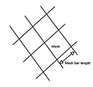
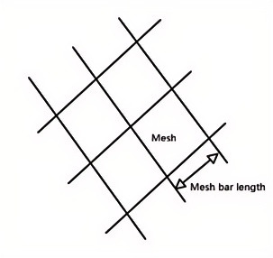
In these equations, S_n represents the net solidity, given by S_n=2R/b, where R is the twine diameter and b is the bar length. The unit cell configuration of the net is illustrated in Figure 1.

Figure 1.Bar length and twine arrangement of the net panel structure.

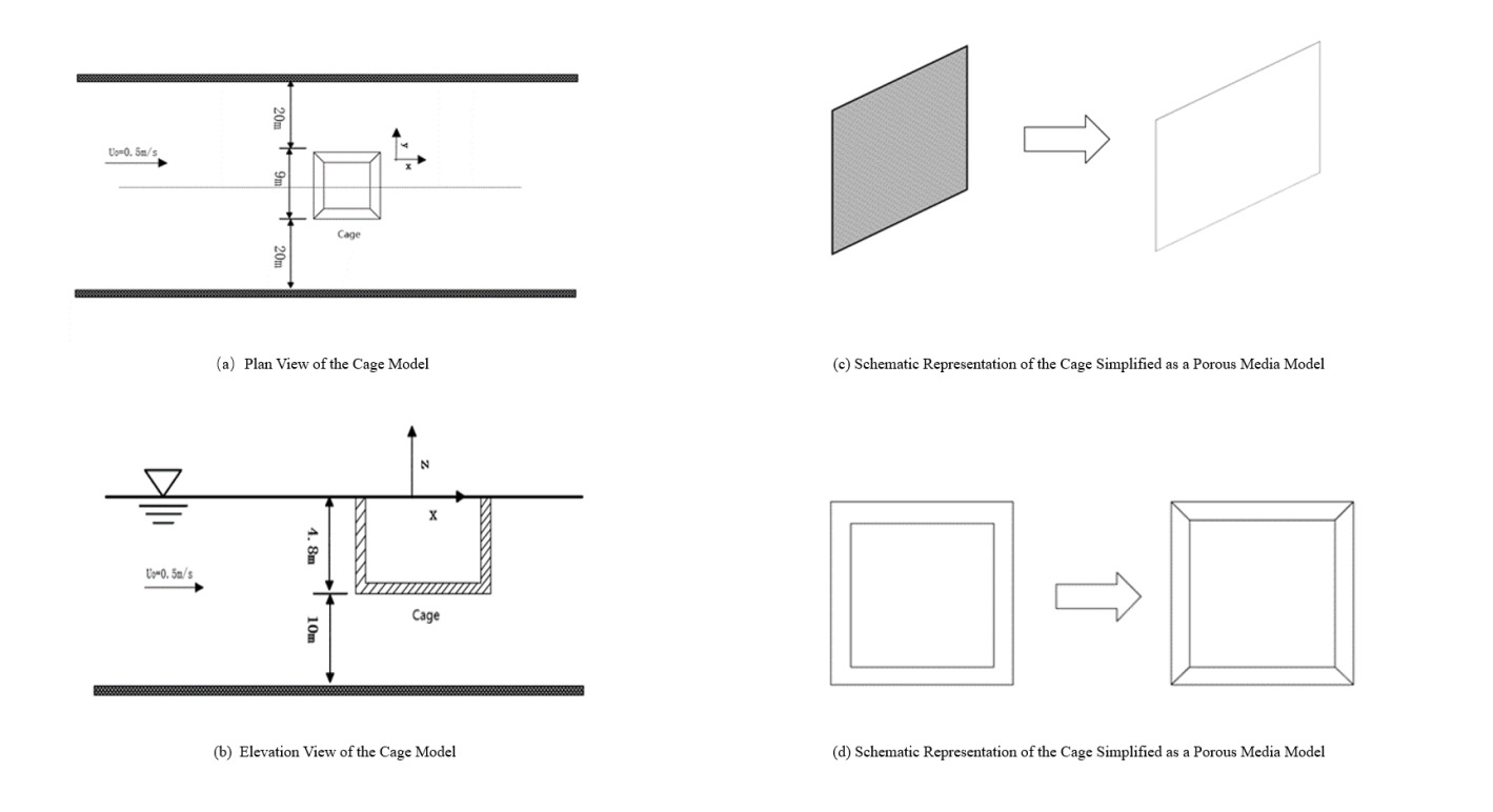
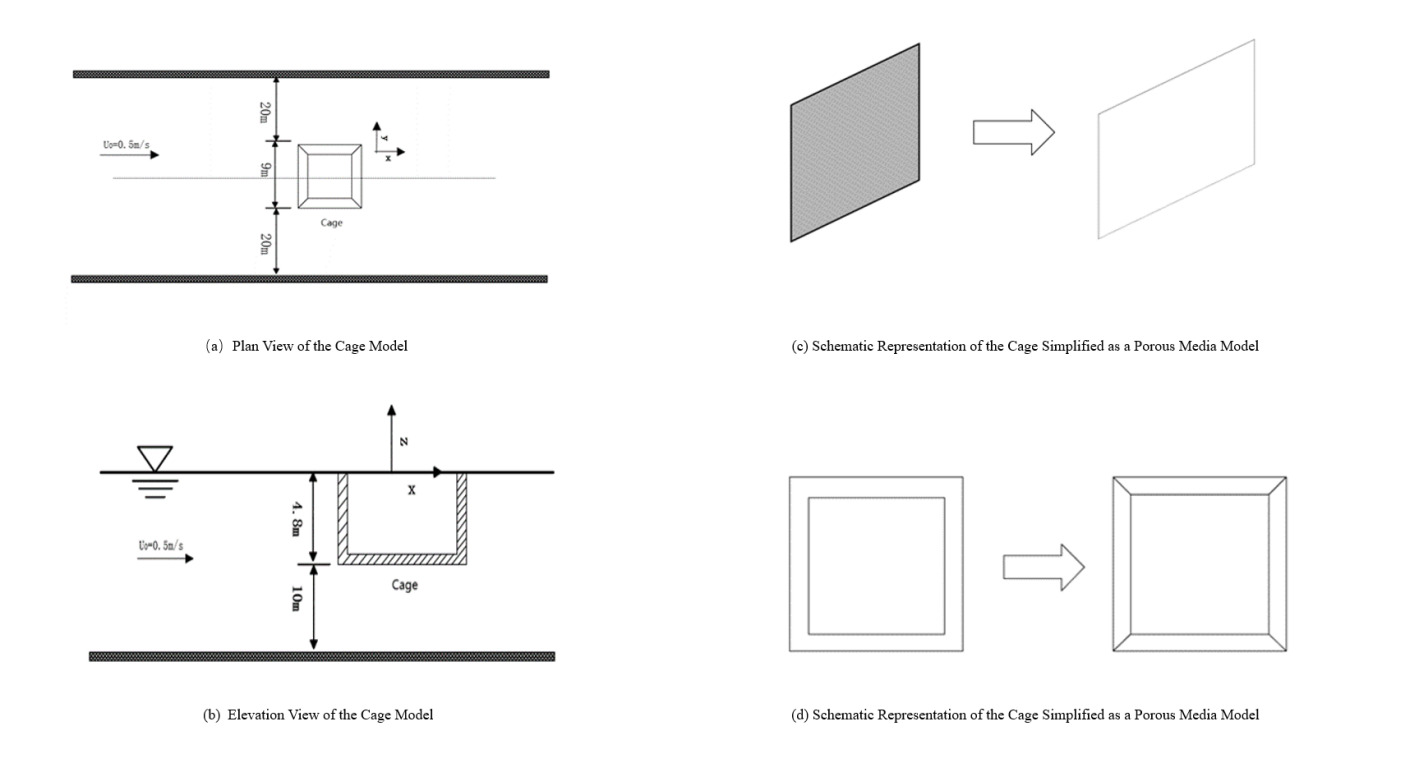
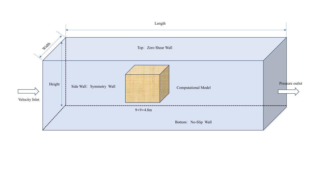
In this study, the fish cage was idealized as a simplified structure comprising five net panels uniformly arranged on a square framework. The hydrodynamic behavior of a single cage was simulated by assigning porous-media parameters to each net panel under different flow incidence angles. A schematic illustration of the cage geometry and its simplified computational model is shown in Figure 2.

Figure 2.Schematic of the simplified cage model

Discrete Phase Model

The Discrete Phase Model^33,34 is suitable for the two-phase flow problem in this study, as the volume fraction of the discrete phase remains below 10%, ensuring its applicability. Within this framework, individual particles are tracked using a Lagrangian formulation, while the continuous fluid phase is resolved through an Eulerian approach by solving the Navier-Stokes equations. This combination enables a two-way coupling between the fluid and particle phases through momentum exchange. The motion of each particle is obtained by integrating the force differential equation in the Lagrangian reference frame. The particle’s force balance, where its inertia equals the total forces acting upon it, can be expressed in Cartesian coordinates as:

\[\frac{du_{p}}{dt} = F_{D}(u - u_{p}) + \frac{g_{X}(\rho_{p} - \rho)}{\rho_{p}} + F_{X}\tag{14}\]

Where FD is the drag coefficient, which can be calculated by:

\[F_{D} = \frac{18\mu}{\rho_{p}d_{p}^{2}}\frac{C_{D}Re}{24}\tag{15}\]

In this formulation, u denotes the fluid velocity, u_p is the particle velocity, μ represents the dynamic viscosity of the fluid, ρ and ρ_p are the fluid and particle densities, respectively, d_p is the particle diameter, and Re refers to the particle Reynolds number, which is defined as:

\[Re \equiv \frac{\rho d_{p}|u_{p} - u|}{\mu}\tag{16}\]

Where C_D is the drag coefficient, which can be expressed by the following relation:

\[C_{D} = a_{1} + \frac{a_{2}}{Re} + \frac{a_{3}}{Re}\tag{17}\]

For spherical particles, the empirical coefficients a₁, a₂, and a₃ in the correlation are considered constants within a specific Reynolds number range.

\[\mathbf{x}_{p}(t) = \mathbf{x}_{p0} + \int_{t_{0}}^{t}\mathbf{u}_{p}(t)dt\tag{18}\]

Where x*_p0* denotes the initial position of the particle, and t₀ represents the initial time, respectively.

The discrete phase model is applicable to particle-laden two-phase flows at low volume fractions, assuming negligible interparticle interactions and that particle motion is primarily governed by fluid forces. Based on this, the sediment is treated as a dilute discrete phase in this study, considering only momentum exchange with the continuous phase.

Boundary Conditions and Numerical Methods

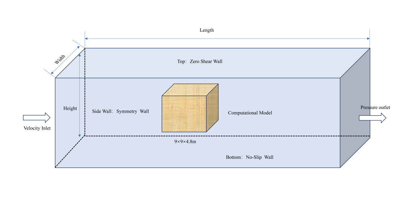
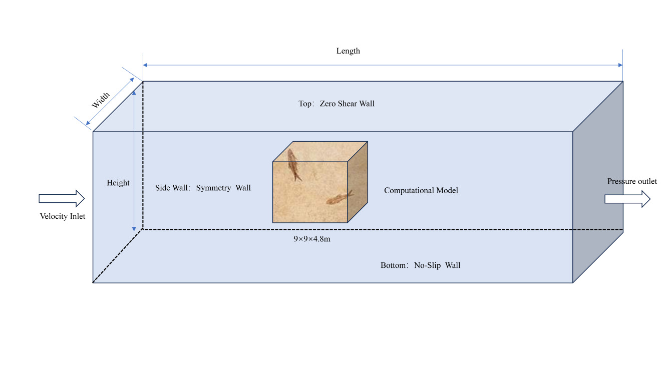
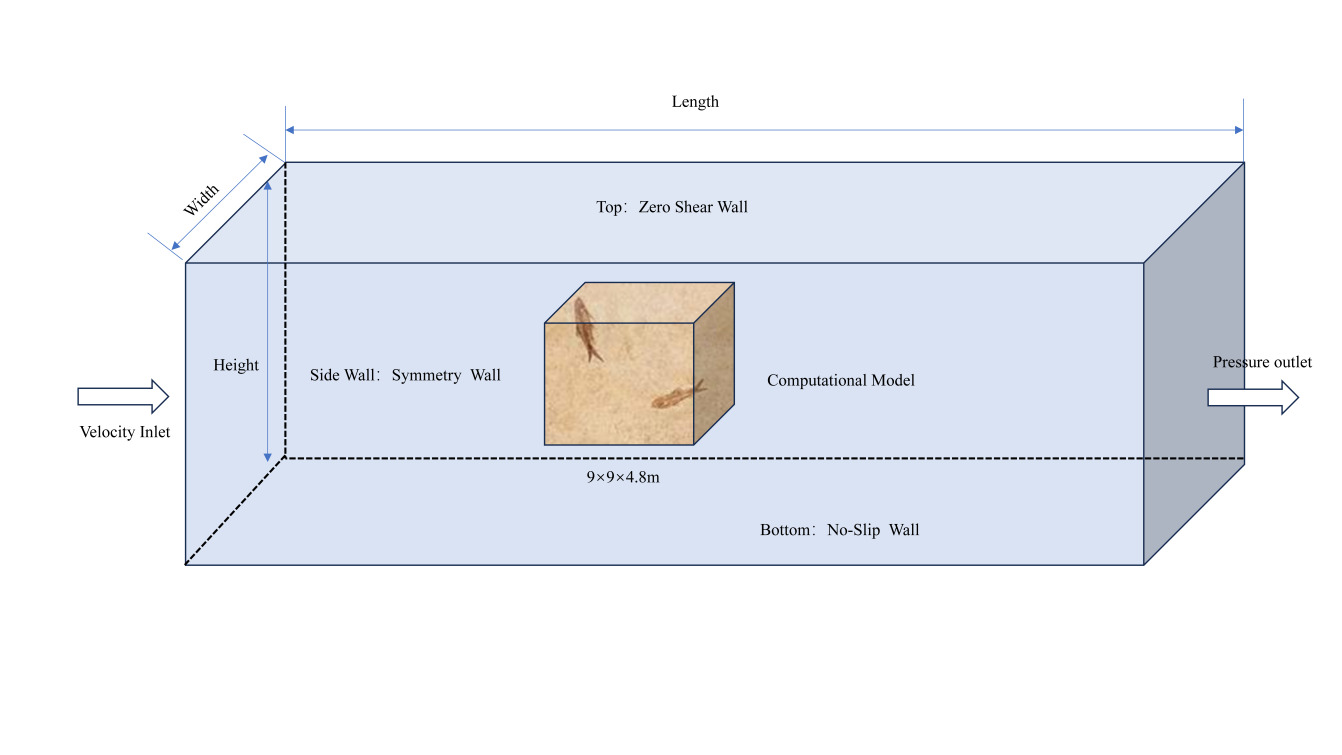
In the numerical setup, a velocity inlet boundary condition was imposed at the upstream boundary of the external domain, while an outflow condition was applied at the downstream boundary to maintain mass conservation and ensure a realistic pressure field. The lateral boundaries were defined as symmetry planes to minimize lateral confinement effects, and the bottom boundary was modeled as a no-slip wall to represent viscous interactions with the seabed. The top surface was treated as a stress-free wall, mimicking the hydrodynamic characteristics of an open sea surface.

For the porous media regions, a porous jump boundary condition was employed to represent the flow resistance equivalent to that imposed by the net panels. In Fluent, anisotropic resistance is achieved by setting direction-dependent resistance coefficients for the porous medium. In the Discrete Phase Model calculations, the particle-boundary interaction at the bottom was defined as a “trap” condition, simulating the deposition process of sediment or other particulate matter.

The particle phase was tracked using a Lagrangian approach, while the fluid phase was solved via an Eulerian framework. The motion of particles is influenced by fluid velocity, pressure, and turbulence. Concurrently, particles exert a reciprocal effect on the fluid phase, primarily through momentum exchange, turbulence modulation, and energy transfer, thereby modifying the continuous phase flow behavior. To accurately capture these fluid-solid interactions, a two-way coupling approach was adopted in the solution.

Flow velocities were recorded at four measurement points located both upstream and downstream of the net panel. These data were used to determine the drag coefficient C_n and lift coefficient C_l of the net. A comparison between the numerical predictions and experimental measurements is summarized in Table 1. The simulated results show strong consistency with experimental observations, with deviations remaining within acceptable error margins. This confirms that the porous media model effectively reproduces the hydrodynamic behavior of the net panel and cage structure, providing a reliable foundation for further flow field analysis of aquaculture cages.

This study adopts a steady-state numerical simulation approach, which does not involve a physical time-marching process. Convergence is determined during the computation using dual criteria of residuals and monitored quantities: the calculation is considered converged when the residuals of the continuity equation, momentum equations, and turbulence equations all drop below 10^-5, and the velocity variations at typical monitoring points inside the cage and in the wake region become stable. Convergence is typically achieved after approximately 2400 iterations. In the discrete-phase calculation, a two-way coupling method is used to account for particle–fluid interactions. The continuous-phase flow field and particle-phase motion are updated alternately until both phases reach steady state, ensuring the reliability of the numerical results.

Model Verification and Validation

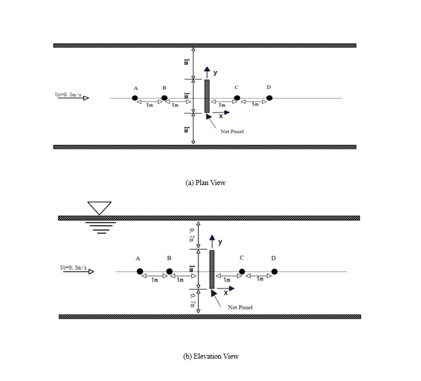
The numerical model was validated against experimental data from Patursson et al. for a single net panel. The comparison is shown in Figure 3. A numerical flume measuring 35 m in length, 4 m in width, and 4 m in depth was used. Bi et al.³⁰ tested three porous media thicknesses: 5 mm, 10 mm, and 50 mm. Results showed that thickness has little effect on the simulation. Therefore, a 50 mm thickness was chosen for the net porous media. This selection balances accuracy and grid size. The twine diameter was 2 mm, and the bar length was 0.028 m. The x-, y-, and z-axes represent the streamwise, transverse, and vertical directions, respectively. A uniform inflow velocity of U₀ = 0.5 m/s was applied at the inlet.

Figure 3.Model and measurement points

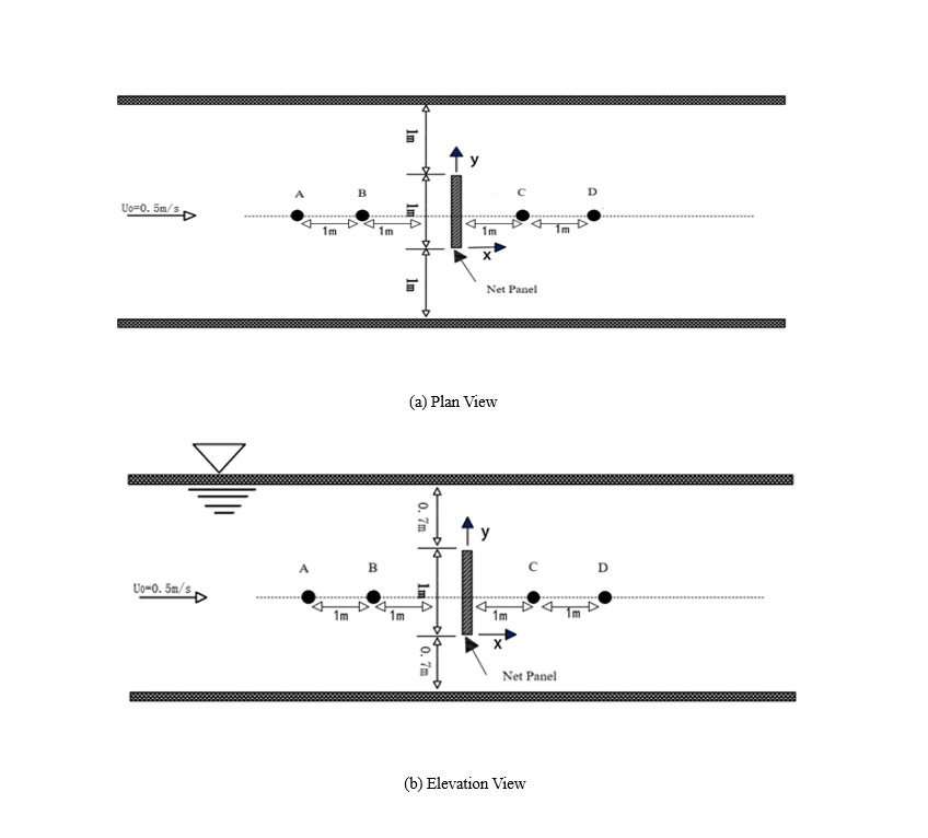
Flow velocities were measured at four monitoring points upstream and downstream of the net panel. These values were used to calculate the drag coefficient C_n and lift coefficient C_l of the net. A comparison between the simulated results and existing experimental data is presented in Table 2. The results indicate that the numerical predictions are in good agreement with the experimental measurements, with discrepancies falling within acceptable limits. This demonstrates that the porous media model reliably captures the flow characteristics around the net panel and the cage structure, thereby providing a sound theoretical basis for subsequent hydrodynamic analysis of the cage system.

The validation conditions in this study use a uniform incoming flow with the netting arranged vertically, aiming to calibrate the porous media model’s ability to characterize the netting’s basic resistance characteristics. These conditions enable accurate determination of the netting’s normal resistance, providing fundamental parameters for complex scenarios. The effects of multiple cages, fish bodies, and sediment primarily alter the local flow-field distribution and momentum-exchange processes, without changing the dominant resistance mechanism of the netting. Therefore, the parameters obtained under these conditions can reasonably support numerical simulations under multi-factor coupled scenarios.

Results

Numerical Simulation of Large Yellow Croaker Aquaculture Net Cage

Description of the Net Cage Case

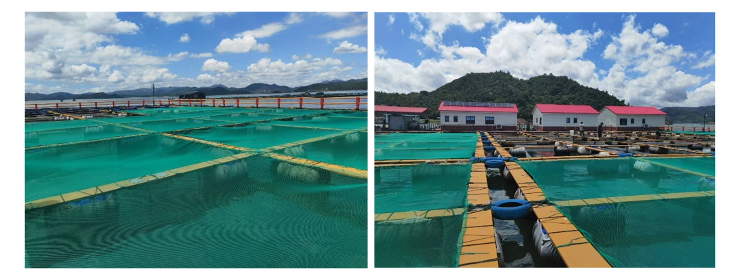
Based on the prototype of a large yellow croaker aquaculture farm located offshore of Ningbo, a geometric and environmental model of the net cage was developed for numerical computation. According to field survey data, As shown in Figure 4, the cage structure is square-shaped, measuring about 9 m on each side and 4.8 m in height. It is constructed using knotless polyethylene netting composed of 2 mm diameter twine with a mesh bar length of 0.028 m. From these parameters, the net solidity is calculated as S_n= 0.143, and the porosity is approximately 0.82. The stocking density is about 9 fish/m³, with an average body weight of approximately 0.5 kg per large yellow croaker during the spring season. To match the actual structural layout, the numerical flume was configured with a length of 150 m, a width of 30 m, and a depth of 30 m. The net cage is positioned at the center of the flume, with its center located approximately 34.5 m from the inlet boundary, ensuring fully developed flow conditions at the cage site.

Figure 4.Aquaculture Net Cage

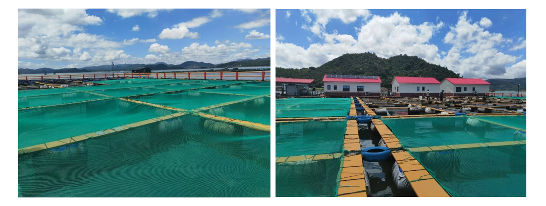
The study area is located in the offshore aquaculture zone near Ningbo, Zhejiang, characterized by a typical subtropical monsoon climate. The region is influenced by both the coastal currents of the East China Sea and surface circulation. The average water depth ranges from 20 to 25 meters, with seabed sediments dominated by silty clay mud. The suspended sediment grain size measures approximately 60-100 μm. Field measurements indicate that tidal dynamics in the area are primarily semidiurnal. The flood and ebb currents mainly follow a northeast-southwest direction, with flow velocities ranging between 0.3-0.7 m/s. A representative inflow velocity of 0.5 m/s was selected for this study. The mean annual water temperature is approximately 20.5°C, with salinity varying between 27-31 PSU. The resulting seawater density ranges from 1023 to 1026 kg/m³.

Modeling, Meshing, and Simulation

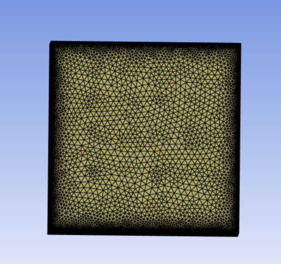
The cage structure was modeled using the DesignModeler module in ANSYS, while the 3D geometry of the large yellow croaker was imported from SolidWorks. An unstructured tetrahedral mesh was employed. The porous media region representing the net panel was discretized with the minimum element size. The mesh size was then gradually increased inward and outward from this region with growth rates of 1.1 and 1.2, respectively. The surface of the large yellow croaker model was meshed,³⁵ while its internal volume was not. In the present study, fish bodies are simplified as stationary rigid structures with no-slip wall boundary conditions. This treatment aims to represent the macroscopic blockage effect and additional flow resistance induced by fish biomass, which are the dominant mechanisms affecting cage-scale hydrodynamics. Although real fish exhibit active swimming behavior, including tail-beat-induced turbulence and schooling dynamics, previous experimental and numerical studies have shown that, at the scale of aquaculture cages, the overall hydrodynamic effect of fish schools can be reasonably approximated as an equivalent resistance or momentum sink.^19,30,35

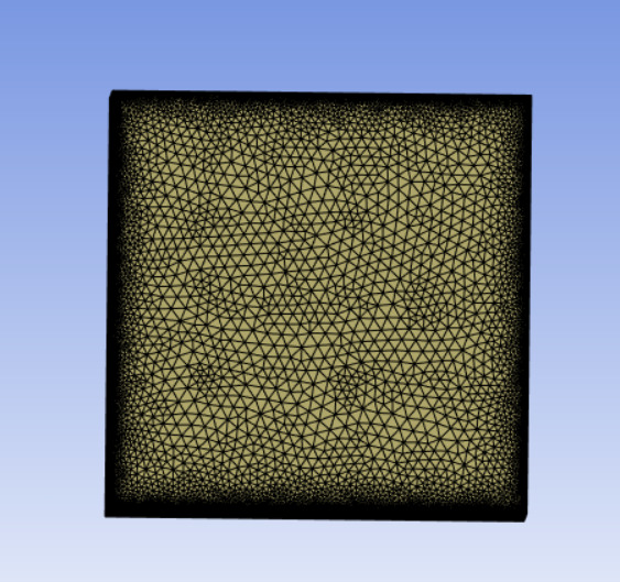
A grid independence study by Zhang et al.³ was conducted using three mesh configurations with minimum element sizes of 0.025 m, 0.020 m, and 0.017 m. The results showed that reducing the element size from 0.020 m to 0.017 m caused less than a 1.8% change in the average flow velocity inside the cage and less than a 2.3% difference in the maximum velocity within the wake region, indicating satisfactory convergence. Consequently, the mesh with a minimum element size of 0.017 m was selected for the final simulations to balance computational accuracy and efficiency. A detailed view of the local mesh is presented in Figure 5.

Figure 5.Schematic Diagram of the Local Mesh for the Net Cage

The inlet boundary was set as a velocity inlet with a flow velocity of 0.50 m/s and a turbulence intensity of 5%. The fluid density was set to 1025 kg/m³, and the dynamic viscosity was 1.08×10^-3 Pa·s. When simulating sediment effects, the Discrete Phase Model was activated with two-way coupling. The sediment density was set to 2650 kg/m³ with a particle diameter of 100 μm, and the injection flow rate was 5×10^-6 kg/s. Particles were injected at the fluid inlet boundary. A mixed “Trap” and “Reflect” condition was applied to the cage and bottom boundaries to simulate the processes of partial deposition and resuspension.

Analysis of Simulation Results

Effect of Net Panels on the Hydrodynamic Performance of the Cage

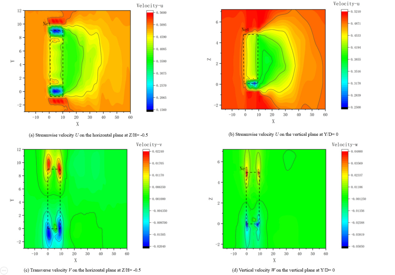
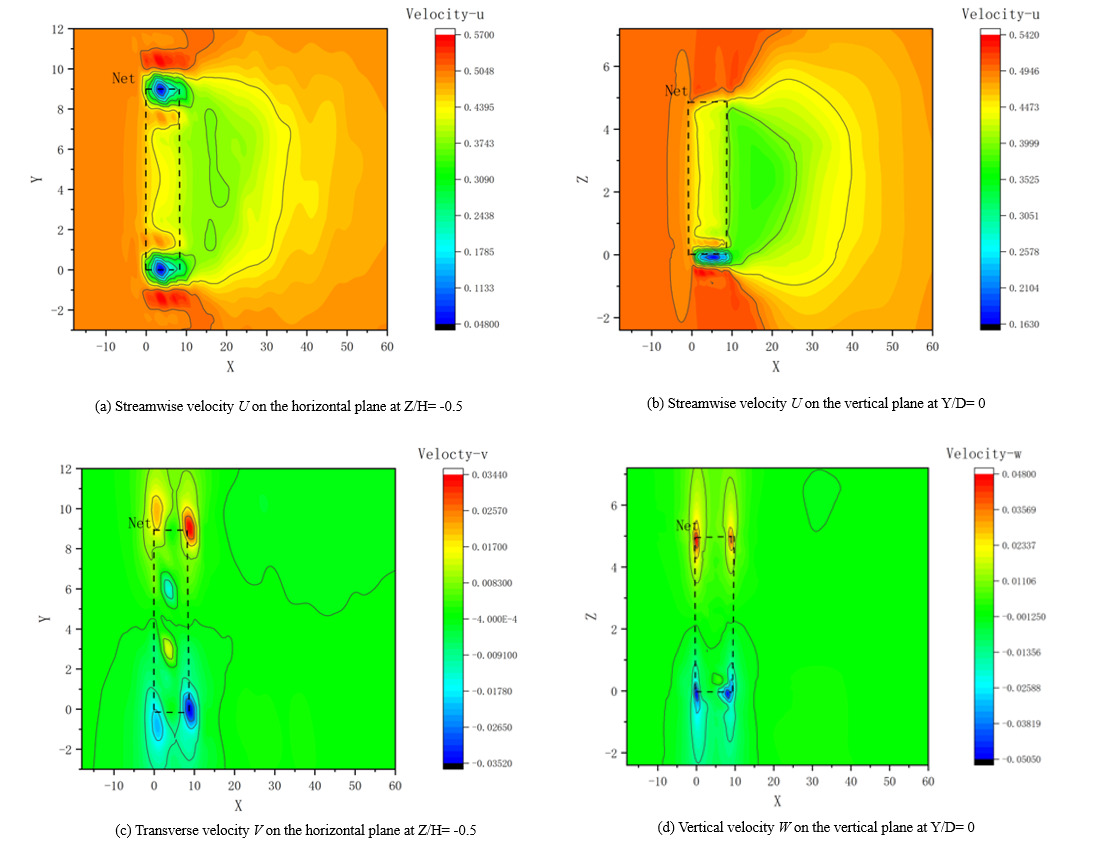
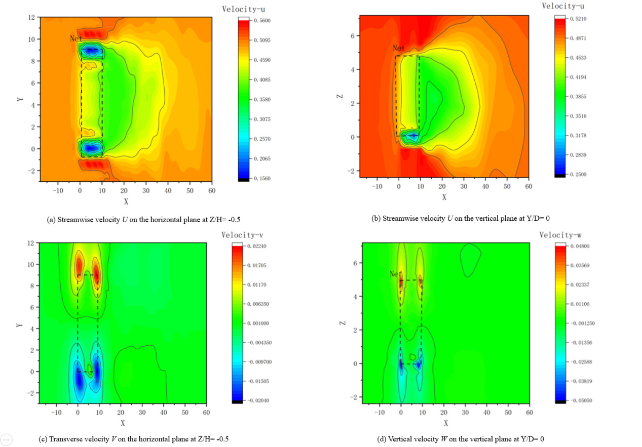
Figure 6 presents the flow field distribution cloud map considering only the effect of the net cage, with the black dot-dash line indicating the spatial position of the cage. Regarding the overall distribution characteristics, the flow is significantly obstructed as it passes through the cage, exhibiting typical leading-edge deceleration and wake attenuation features. Due to the flow resistance imposed by the net panels, a localized velocity reduction zone forms upstream of the cage, with notably weakened internal flow velocity. A large-scale wake attenuation zone develops downstream, accompanied by a certain degree of flow recirculation. Simultaneously, influenced by flow-around effects, the velocity increases markedly along the sides of the cage, forming clearly visible localized acceleration regions.

Figure 6.Schematic of the experimental model considering only the netting

Analysis of the velocity components reveals a distinct three-dimensional flow pattern inside the cage. The maximum transverse velocity V_max occurs on the sides of the cage, accelerating to 0.0224 m/s, which is approximately 4.48% of the incoming flow velocity U₀. The maximum vertical velocity W_max appears beneath the cage, reaching 0.041 m/s, or 8.2% of U₀. This indicates that the drag force of the net panels not only alters the streamwise velocity distribution but also induces significant transverse and vertical flow disturbances.

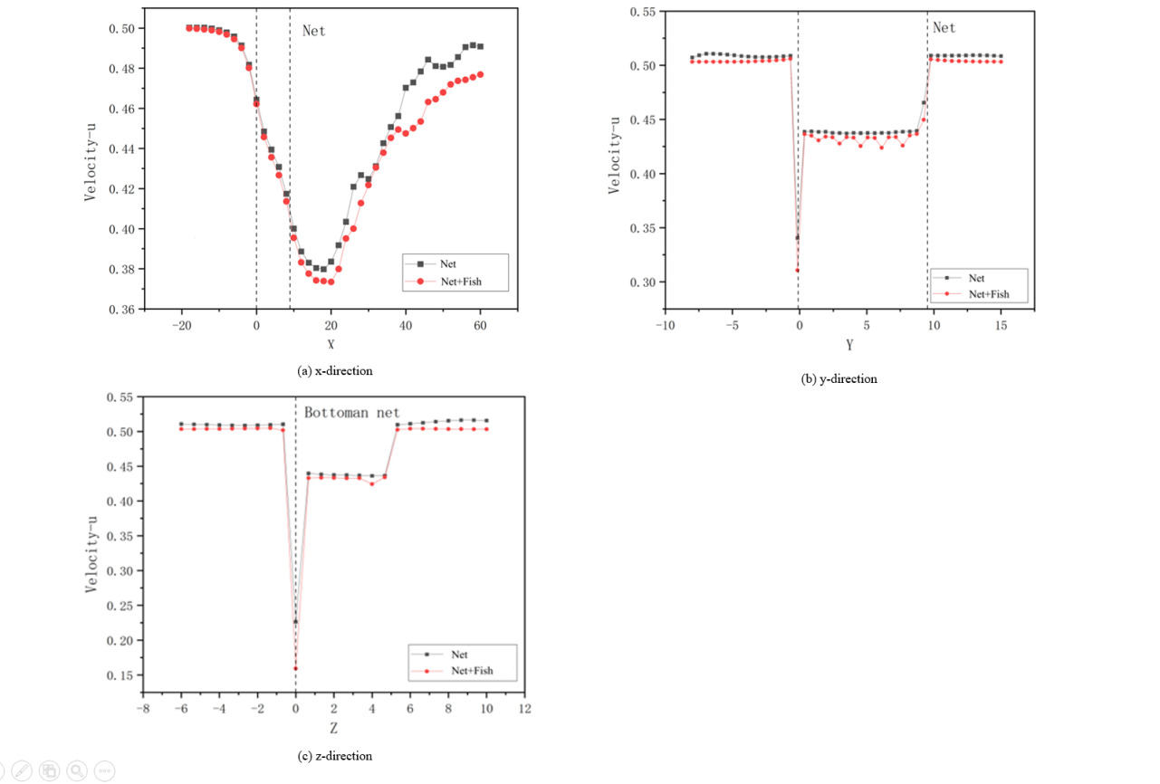
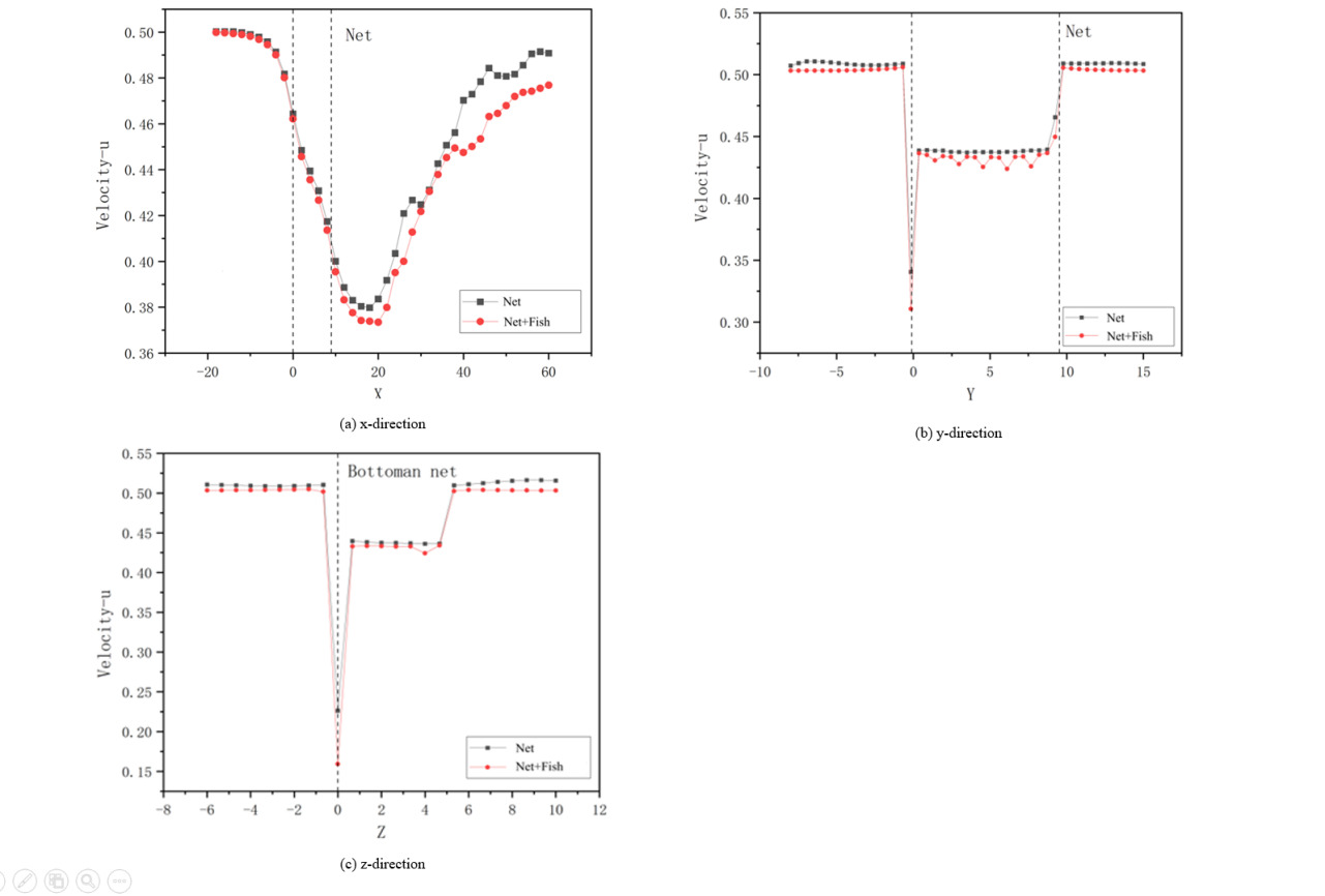
The variation curve of the streamwise velocity U is shown in Figure 7 and Tables 3-5. In the flow direction, the velocity gradient is greatest at the cage edges (Y/D=0.5, Z/H=-0.5), indicating intense local shear effects. After passing through the cage, the flow velocity decreases sharply, dropping to a minimum of 0.41 m/s inside the cage, which is about 82% of the incoming flow velocity. The wake then begins to recover, gradually approaching the incoming flow velocity at approximately 2 cage diameters downstream.

Figure 7.Variation of the streamwise velocity U along different directions

Observing the transverse direction (y-direction), the streamwise velocity at the cage center decreases to 0.44 m/s (about 88% of U₀), while it accelerates to 0.51 m/s (about 1.02 U₀) on the sides due to the flow-around effect, demonstrating a clear velocity stratification. Along the vertical direction (z-direction), the velocity gradually decreases from 1 m below the cage to the cage bottom, reaching a minimum of 0.16 m/s at the bottom (about 32% of U₀). The velocity attenuation is more pronounced closer to the cage center. After the fluid passes through the cage, the velocity gradually recovers, approaching the incoming flow velocity again at 1 m above the cage top.

The wake attenuation range simulated in this study closely corresponds to the numerical and experimental results reported by Zhao et al.²² further confirming the applicability and accuracy of the porous media model in net panel flow analysis. Xu et al.³¹ demonstrated that the local resistance distribution of netting is strongly correlated with turbulent flow structures and significantly affects wake velocity recovery. Meanwhile, Zhao et al.²² observed a velocity reduction of approximately 15-25% inside cages under comparable Reynolds number conditions, which aligns well with the patterns identified in our study.

Beyond confirming existing knowledge, this work provides new insights into the detailed vertical velocity distribution within the cage. The results reveal that net panel resistance not only attenuates flow in the main streamwise direction but also enhances local vertical flows and redistributes energy, generating fine-scale vortex structures and shear-induced stratification in the downstream region. These findings highlight the continued advantage of the porous media model in resolving three-dimensional flow features and suggest its novel application value for quantitatively characterizing local flow disturbances around aquaculture cages.

These findings collectively demonstrate that net panels are a critical structural element governing cage hydrodynamics, with their geometric parameters directly determining wake velocity distribution and turbulence intensity variations. The numerical approach employed here enables quantitative analysis of flow variations in different regions around the cage, providing fundamental data for subsequent investigations into fish behavior interactions and sediment transport processes.

Coupled Effects of Large Yellow Croaker on Cage Hydrodynamics

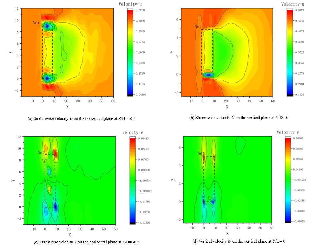
Figure 8 illustrates the three-dimensional flow field distribution under the combined influence of fish and the cage structure, with the black dot-dash line indicating the cage position. The numerical results show that the overall flow pattern remains broadly consistent with the net-only case, exhibiting distinct wake effects and velocity attenuation zones. However, due to the additional drag imposed by the individual fish, the fluid experiences further kinetic energy loss when passing through the cage, resulting in more significant velocity attenuation inside and downstream of the cage, as well as increased complexity in the flow structure.

Figure 8.Variation of the Streamwise Velocity U along Different Directions

Specifically, the maximum transverse velocity V_max=0.035 m/s, representing about 7% of the incoming velocity U₀, while the maximum vertical velocity W_max=0.050 m/s, accounting for 10% of U₀. Compared to the net-only scenario, the inclusion of fish bodies introduces noticeable fluctuations in the velocity distribution inside the cage and enhances local vortex structures.

Figure 9 and Tables 6-8 present comparative profiles of the streamwise velocity through the cage center. The velocity inside the cage decreases to 0.41-0.42 m/s, corresponding to 82%-84% of U₀, with a wake attenuation magnitude of up to 16% downstream. In the net-only case, the wake velocity recovered to about 98% of U₀ at approximately 6 cage diameters downstream. However, when large yellow croakers at 5% of the actual stocking density are included, the velocity at the same location only recovers to 0.96U₀, indicating that the presence of fish significantly prolongs the wake recovery distance.

Figure 9.Flow velocity patterns within and surrounding the aquaculture net cage

Along the y-direction, the arrangement of fish induces periodic fluctuations in the streamwise velocity within the central region of the cage, where the local velocity drops to a minimum of 0.42 m/s, or about 0.84U₀. In the z-direction, velocity attenuation near the bottom is particularly pronounced. Without fish, the minimum velocity was about 55% of U₀, which further decreases to 68% when fish are added, indicating inhibited fluid exchange near the seabed.

Compared with the findings of XU et al.³¹ and Patursson et al.¹⁰ the wake attenuation patterns observed in this study are generally consistent: the combined resistance of the cage structure and fish collectively attenuates the incoming flow kinetic energy, intensifies local turbulent structures, and extends the length of the wake recovery region. However, the predicted flow velocity attenuation in this study is slightly stronger, and the wake recovery distance is longer, attributable mainly to the following three aspects.

First, differences in fish modeling approaches contribute to the deviation. This study simplifies the large yellow croaker as rigid bodies and does not account for the additional kinetic energy feedback induced by tail beating during actual swimming. Existing research indicates that fish swimming can generate induced flows in local regions, thereby reducing velocity attenuation in the wake zone. Second, discrepancies exist in the resistance parameter settings for the net panels. The normal and tangential resistance coefficients selected in this study are taken from the upper range of measured values, leading to relatively higher local resistance in the simulation and thus enhanced flow attenuation. In contrast, the lower solidity conditions adopted by Tsukrov et al.⁶ and Xu et al.³¹ result in smaller resistance coefficients and consequently faster wake recovery. Finally, differences in the turbulence model and incoming flow Reynolds number also affect wake prediction accuracy. This study employs the Realizable k-ε turbulence model, which exhibits strong turbulent dissipation capability in high-Reynolds-number flows, leading to a relatively slower velocity recovery in the downstream region.

In summary, the simulation results of this study align well with previous experimental and numerical findings in overall trends, validating the reliability of the established coupled model. Moreover, this work provides quantitative insights into the influence of fish distribution on the internal vertical flow structure of the cage, revealing that fish resistance not only enhances local turbulent disturbances but also generates a wake dominated by energy dissipation downstream. These findings offer critical theoretical and practical implications for optimizing stocking density, improving cage structural design, and enhancing water exchange efficiency.

Effect of Sediment Particles on Cage Hydrodynamics

It should be noted that the objective of this study is to evaluate the incremental effect of sediment under realistic aquaculture conditions, where fish and netting coexist. Therefore, the “netting–fish” case is treated as the baseline condition, and the “netting–fish–sediment” case reflects the actual environmental scenario. As a result, the influence of sediment is interpreted as a background-dependent response rather than an isolated effect. Although a “netting–sediment” case could further separate independent contributions, its absence does not affect the validity of the present conclusions regarding flow modification under practical farming conditions.

When considering the combined effects of fish, cage structure, and sediment particles, the numerical simulation results reveal that the flow field exhibits more complex multiscale coupling, as shown in Figure 10. Overall, the macroscopic distribution pattern of the flow field remains dominated by the cage structure. However, the superposition of the volume-blocking effect from fish bodies and the momentum feedback effect from sediment particles results in a more non-uniform velocity distribution inside and downstream of the cage, with significantly enhanced turbulent structures.

Figure 10.Flow velocity patterns within and surrounding the aquaculture net cage

In terms of velocity component variations, the maximum transverse velocity V_max is 0.028 m/s, approximately 5.56% of the incoming flow velocity U₀, while the maximum vertical velocity Wmax reaches 0.235 m/s, accounting for 47% of U₀. Compared to the scenario considering only the net panel, the resistance from fish further attenuates the flow velocity inside the cage, while the presence of sediment particles, through two-way fluid-particle momentum coupling, locally enhances the re-acceleration phenomenon in the wake region. This results in a stratified velocity distribution: significant flow reduction in the upper part of the cage and local flow recovery in the lower sediment settlement zone.

Figure 10 and Tables 9-11 present comparative results of the streamwise velocity distribution profiles through the cage center. Compared to the case considering only the net panel and fish, the inclusion of sediment reduces the streamwise velocity U inside the cage by approximately 12%-15% overall. However, in the downstream wake region within about 5-7 cage diameters, local recovery occurs, with velocity restoring to 98%-99% of the incoming flow velocity. This recovery is slightly higher than the 96% observed in the case with only fish and net panel, indicating that sediment introduction alters the momentum distribution and turbulent dissipation characteristics in the wake region.

The streamwise velocity variation curves through the cage center were compared with corresponding cases involving only the net panel and the net panel with large yellow croaker. It can be observed that the streamwise velocity distribution when considering fish, sediment, and net panel together is similar to that of the net panel-only case. However, the flow velocity downstream of the cage is higher than in both the net panel-only case and the case with net panel and fish combined.

This phenomenon is consistent with the findings of Xu et al.³¹ and Liu et al.¹³ both indicating that particles exhibit significant inertial lag effects in the flow field. Their momentum feedback can create localized “re-acceleration” zones in the wake region, leading to a recovery trend in downstream flow velocity.

Comprehensive analysis reveals three primary mechanisms responsible for the local velocity recovery in the wake region: Momentum Feedback Mechanism: When sediment particles enter the low-velocity wake zone, their velocity lags behind the main flow, significantly reducing the reverse drag force on the fluid. This decrease in local resistance induces slight re-acceleration within the wake core region.Turbulent Redistribution Effect: Sediment particles trigger secondary turbulence within the wake shear layer, altering the spatial distribution of turbulent energy. This redistribution concentrates part of the turbulent kinetic energy back into the mainstream direction, thereby enhancing velocity recovery capability in the wake region. Density Difference and Particle Settling Effect: The settling of sediment particles in the wake region increases local fluid density in the lower layers, subsequently modifying pressure gradient distribution. Upper-layer fluids accelerate as they circumvent these high-density zones, forming localized velocity recovery bands.

This study not only confirms the momentum feedback characteristics of sediment particles but also further reveals the nonlinearly enhanced redistribution effect in the wake under the synergistic action of fish and sediment. The results demonstrate that when fish and sediment coexist, the wake recovery velocity increases by approximately 6-10% compared to the cage-only scenario, with local turbulent kinetic energy enhanced by about 15%. Nevertheless, the overall flow attenuation remains predominantly governed by the structural resistance of the cage.

Analysis of Results

Simulation results indicate that the presence of netting significantly dissipates incoming flow energy, resulting in a velocity reduction of approximately 15%–25% in the wake region and the formation of a relatively stable downstream recirculation zone. These findings are consistent with both experimental and numerical results reported by Fan et al. and Zhao et al., confirming the reliability and applicability of the porous media model for simulating the hydrodynamic behavior of aquaculture cages.

When both fish bodies and netting are considered, the overall flow distribution remains primarily governed by the drag of the net structure. However, additional resistance from the fish and the associated flow separation significantly intensifies local turbulence. Numerical results show that the maximum lateral and vertical velocities reach approximately 7% and 10% of the inflow velocity, respectively, while the wake decay region expands and the downstream recovery distance increases by about 10%. These trends agree with the results of Xu et al.³¹ and Liu et al.,¹³ although the present study predicts slightly higher attenuation. This difference is mainly attributed to the use of relatively high porous resistance coefficients and the assumption of rigid fish bodies, both of which enhance local energy dissipation. The results suggest that the presence of fish redistributes energy within the cage, leading to a non-uniform, dissipation-dominated wake structure.

When the combined effects of fish, netting, and sediment are considered, the flow field exhibits a more complex coupled response characterized by momentum feedback and turbulent energy redistribution. Momentum exchange between sediment particles and the surrounding fluid generates localized “re-acceleration zones” downstream, increasing flow velocity by approximately 6%–10% and enhancing turbulent kinetic energy by about 15% compared with the single-cage scenario. This behavior can be attributed to the combined effects of momentum feedback, turbulent energy redistribution, and density gradient variations, indicating that moderate sediment concentrations can promote wake recovery. The present findings not only support the particle lag and momentum feedback mechanisms proposed by Fan et al. and Li et al., but also suggest a coupled enhancement effect in wake redistribution under fish–sediment interactions.

In summary, this study systematically elucidates the coupled hydrodynamic mechanisms among netting, fish bodies, and sediment within aquaculture cages, clarifying their dominant and interactive roles in flow regulation. The results provide theoretical and engineering insights for optimizing deep-sea cage design, regulating stocking density, and improving water exchange efficiency in intensive mariculture systems.

Discussion

This study established a three-dimensional hydrodynamic model based on a porous media approach to investigate the flow field inside and around a large yellow croaker aquaculture net cage. Numerical simulations were conducted for three scenarios: net panel only, net panel with fish, and net panel with both fish and sediment. The hydrodynamic characteristics and wake behavior around the cage were systematically analyzed.

The main conclusions are as follows:

1. The porous media model can effectively reproduce the flow field characteristics around large-scale aquaculture net cages.

2. The net panel is the primary factor influencing overall flow resistance and velocity distribution, leading to wake velocity reduction and enhanced flow disturbances.

3. Under the net panel-only condition with a solidity s_n = 0.143, the main flow direction remains largely unchanged. However, the transverse velocity V and vertical velocity w reach maximum values around the cage, accounting for approximately 4.48% and 6.2% of the incoming flow velocity, respectively. The velocity attenuation at the cage center reaches about 10%, while downstream velocity initially decreases, with a maximum attenuation of approximately 18%, and gradually recovers to the incoming flow level at around two cage diameters downstream. Additionally, the flow velocity near the cage bottom slightly increases by about 1%–2% compared to the incoming flow. These results indicate that the net panel significantly influences local flow disturbances and velocity distribution, while having minimal impact on the overall flow direction.

4. When both fish and net panel are considered, the overall flow pattern remains similar to that of the net panel-only case, with pronounced wake effects. However, due to the additional drag induced by fish, velocity attenuation inside and downstream of the cage is significantly enhanced, and the wake region becomes larger and more intense. The maximum transverse velocity V increases to about 7% of the incoming flow velocity, while the maximum vertical velocity w reaches approximately 10%. Compared with the net panel-only scenario, downstream velocity attenuation is more severe, recovering to only about 96% of the incoming velocity at six cage diameters downstream. Moreover, significant velocity fluctuations occur inside the cage, and bottom velocity attenuation increases to approximately 68%. These findings demonstrate that considering the net panel alone is insufficient to accurately describe the flow characteristics and that the combined effects of fish and net panel must be included.

5. When fish, net panel, and sediment are considered simultaneously, downstream velocity attenuation is reduced. In the DPM, under two-way coupling, sediment particles exchange momentum with the fluid. As particles pass through the net panel and downstream region, part of their momentum is transferred back to the fluid, resulting in localized velocity increases. At higher sediment concentrations, enhanced particle inertia promotes the formation of local acceleration zones downstream. Furthermore, particle–fluid interactions increase turbulent kinetic energy, enhancing mixing and energy redistribution. This leads to stronger turbulent diffusion and reduced velocity attenuation, or even local velocity recovery in the wake region. The presence of sediment also modifies the wake shear layer, promoting lateral high-velocity flow toward the wake center and thereby increasing the velocity in the wake core.

The present model assumes clean netting with a constant solidity of S_n=0.143, corresponding to a porosity of approximately 0.82, and fixed hydrodynamic resistance parameters. Under actual marine aquaculture conditions, however, biofouling can progressively accumulate on cage netting and alter its effective solidity, porosity, and hydrodynamic resistance. Such changes may further affect water exchange, velocity attenuation, turbulence development, and wake recovery around the cage. Therefore, the hydrodynamic responses predicted in the present study may differ from those of cages subjected to different degrees of biofouling.

Although biofouling was not explicitly incorporated into the present model, the existing netting-fish-sediment coupling framework provides a basis for further extending the model to more realistic aquaculture conditions. Future studies should consider different degrees and spatial distributions of net biofouling and incorporate their effects on netting resistance into the coupled framework. This would allow a more comprehensive assessment of the hydrodynamic performance and environmental conditions of marine aquaculture cages under long-term operational conditions.

Overall, the results indicate that neither the net panel nor fish alone can fully characterize the actual flow field within aquaculture cages. Instead, the coupled effects of fish activity and sediment transport should be considered comprehensively. The multi-factor coupled modeling framework proposed in this study provides theoretical support and a numerical basis for optimizing cage design, improving water exchange efficiency, regulating stocking density, and evaluating environmental carrying capacity.

Acknowledgments

This work was supported by the Fishery Administration Project (D8021210076). The funders had no role in study design, data collection and analysis, the decision to publish, or the preparation of the manuscript.

Authors’ Contribution per CRediT

Formal Analysis: Shuang Liu (Equal), Zuwei Cao (Equal), Chao Lyu (Equal). Investigation: Shuang Liu (Equal), Zuwei Cao (Equal), Chao Lyu (Equal). Resources: Shuang Liu (Lead). Writing – original draft: Zuwei Cao (Lead). Conceptualization: Chao Lyu (Lead). Methodology: Chao Lyu (Lead). Writing – review & editing: Chao Lyu (Lead). Funding acquisition: Chao Lyu (Lead). Supervision: Chao Lyu (Lead).

Ethical Conduct Approval – IACUC

No Animal Ethics approval was needed for this work.

Competing of Interest – COPE

The authors declare that they have no known competing financial interests or personal relationships that could have appeared to influence the work reported in this paper.

Informed Consent Statement

All authors and institutions have confirmed this manuscript for publication.

Data Availability Statement

All are available upon reasonable request.